Chromatin structure inference from probabilistic modeling of eigenvectors from Hi-C data analysis in a Bayesian framework
Modeling eigenvectors from Hi-C analysis with spatial depency in a Gaussian Random Walk and infering a latent compartment assignment to A or B as an excuse to master PyMC
Here, I aim to do probabilistic modeling of eigenvectors obatained from the ICE method in Hi-C analysis. The idea is to capture some of the variance lost when hard-labeleling the bins based on only the sign of the eigenvector.
This model infers A/B chromatin compartment structure from the first eigenvector (E1) of the Hi-C contact matrix using a Bayesian framework.
Goals
Replace hard sign-thresholding of E1 with a probabilistic compartment assignment.
Quantify uncertainty in compartment calls for each genomic bin.
Allow for modeling of missing E1 values due to low signal.
Assumptions
Each bin belongs to one of two latent states: A or B compartment.
E1 values are generated from Gaussian distributions specific to each compartment.
Prior belief: A has positive E1 values (\(\mu = 0.5\)), B has negative (\(\mu = -0.5\)).
Bins are initially treated as independent
Spatial depency are added later (Gaussian Random Walk)
Keywords
Gaussian Random Walk, Bayesian MCMC, Chromatin Structure in spermatogenesis
Introduction
Chromatin architecture is of high interest in molecular biology, and increasingly so in molecular evolution. A high-throughput method for mapping the 3D organization of the genome was proposed by Lieberman-Aiden et al. (2009), and has since been the standard method of infering chromatin compartments (Lajoie, Dekker, and Kaplan 2015). Briefly, chromatin interactions from Hi-C sequencing is used to generate an interaction matrix of valid Hi-C contacts, and PCA is performed on the covariance matrix of the observed/expected matrix. The following rationale is proposed and experimentally supported; if clustering into 2 types (A/B compartments), genomic positions that interact will yield a positive value in the covariance matrix, and vice versa for positions that do not interact. Then, when PCA is performed, the first principal component captures the variance that arise from being in different compart by its sign. The direction of the eigenvector (the sign) is then phased with a biologically relevant measure (such as GC content) to establish that the A compartment is largely the active chromatin and B is largely inactive.
However, this approach may place too much confidence in how expected interaction frequencies are estimated. By using the eigenvectors within a probabilistic model, where compartment identity is treated as a latent variable, we aim to recover information discarded in hard-labeling based on eigenvector signs. We propose a Bayesian MCMC framework as a spatially aware clustering method that soft-assigns compartments based on the eigendecomposition by assuming that the magnitude of the eigenvector is significant.
Bayesian Statistics and modeling
I Bayesian statistics, a prior belief, \(P(\theta)\) is combined with the likelihood of observed data, \(P(D|\theta)\), to achieve a posterior probability, \(P(\theta|D)\), as Bayes’ Theorem formulates in
which integrates the likelihood over all possible parameter values, weighted by the prior. However, \(P(D)\) is often high-dimensional and therefore intractable to evaluate analytically. Therefore, we can estimate posterior properties without explicitly computing \(P(D)\) by sampling from the posterior using Markov Chain Monte Carlo (MCMC) methods.
MCMC avoids the daunting integral by constructing a Markov chain [ref] with a stationary distribution \(P(\theta|D)\). Then, after a burn-in period, the samples, \(\theta^{(1)}, \dots, \theta^{(N)}\), can be used to approximate the expectation:
\[
\mathbb{E} \left[ f(\theta) \ | \ D \right] \approx \frac{1}{N}\sum_{i=1}^N f \left ( \theta^{(i)} \right ).
\tag{3}\]
This enables us to perform inference in models without analytical evaluation.
Continuing from where we left
This study is a continuation of Chromatin Compartments and Selection on X (MSc thesis) [ref] and some methods were developed there. Especially, one product of the previous study was a pipeline to generate eigenvectors for binned genomes from raw Hi-C reads, utilizing pairtools [ref] cooler [ref] and cooltools [ref] from the Open Chromosome Collective ecosystem [ref].
NB: limitations of using the magnitude of the eigenvector in opposite to only the sign
Methods
```{python}import pymc as pmimport pytensor.tensor as ptprint(pm.__version, pt.__version__)```
The pipeline from [ref] was reused in a modified form to accomodate a new data set of single-cell Hi-C sequencing of human cells. Here, an additional pooling step was introduced to generate merged Hi-C matrices after grouping the samples into two groups established in the sequencing study; the sex chromosome was determined either X or Y. Additionally, it was modified to accomodate the new telomere-2-telomere assembly of Macaca mulata, as it was only available from NCBI, and not UCSC servers.
Data generation
The ICE-method
The pipeline previously developed implements the Iterative Correction and Eigendecomposition (ICE) method of Hi-C analysis (Lieberman-Aiden et al. 2009) after mapping raw Hi-C reads to the reference genome, validating Hi-C pairs, and constructing the interaction map (Hi-C matrix). It is implemented fully using the Open2C tools and recommendations. Briefly, the raw read pairs are mapped (as paired-end reads) to the respective reference genome (either GRCh37 or T2T-MMU8v1.0) with bwa-mem2 [ref] with the -P option. Then the pairs are parsed and sorted with pairtools, and a deduplication and quality filter (\(mapq \geq 30\)) is run to remove PCR duplicates and technical noise from low-quality reads. Lastly, the binned interaction matrices (.cool files, hence also coolers) are created from the remaining pairs into the base-resolution of 1kb bins that is then recursively coarsened until 1 Mb bins. The resulting raw interaction matrices do not have a uniform coverage profile along the genome as a result of differential binding or accesibility of the restriction enzyme and other technical factors. High or low coverage is visible in the interaction matrices, where genomic regions will appear as highly or weakly interacting regions even though they are artefacts of the coverage. Thus, it is needed to balance the interaction counts to avoid visibility-induced biases [ref]; it is time for ICE.
The interaction counts of each bin is corrected iteratively until convergence of the coverage, and the correction weight is saved to the cooler. The expected interaction matrix is derived from the decay in contact probability over genomic distance (also; distance decay), and is used to scale the observed interactions before performing eigendecomposition on the correlation matrix of observed/expected. Bins interacting with bins of the same type should keep a positive eigenvector, and vice versa otherwise. Thus, the first principal component should capture the variance explained by the compartment assignment. The eigenvectors are then oriented to correlate with GC content, to ensure that positive values represent A-compartments and active chromatin, and negative values represent B-compartments and inactive chromatin.
As also described in [ref], sometimes there is a larger amount of variance in interaction frequency between chromosome arms than within arms. In these cases, the eigendecomposition will not capture the compartments, but only change its sign at the centromere. Thus, it is a safe practice to do the eigendecomposition on the chromosome arms separately, and is readily implemented into cooltools by providing a viewframe to the function that does the calculations. It is not clear how further experimentation with narrowing the eigendecomposition viewframe affects the biological explanation of the results, but it is suggested as a method of obtaining more local compartmentalization (Wang et al. 2019) (termed local PCA).
First, the pipeline was applied to generate high-resolution eigenvector tracks on the most recent, telomere-to-telomere Macaca mulata assembly, T2T-MMU8v1.0 [ref], to improve the accuracy of the mapping from the previous study.
Additionally, the pipeline was applied to generate a eigenvectors of human sperm cells harboring the X chromosome. Even though the authors [ref] of this Hi-C data find high similarity between sperm cells harboring the X or the Y sex chromosomes, they barely describe their comparison. Thus, I decide to seperate them into two groups to be able to compare autosomal chromatin compartments later on if we wish to. A major downside of this is that the coverage is approximately halved, resulting in lower viable resolutions for subsequent analyses.
The results of the eigendecomposition are hereafter described as E1 (eigenvector track of the first principal component).
Modeling
I use PyMC (Abril-Pla et al. 2023) for all modeling, relying as much as possible on functions and built-in functionality for all anaysis. I start out small in the simplest model possible, then progressing to larger and more complex models. The basis of the probabilistic modeling is the assumption that the eigenvectors of A- and B-compartments can be drawn from distinct distributions. I assume that the distributions underlying the compartments are Gaussian with different means, either \(\mu_a = 0.5\) or \(\mu_b = -0.5\). Additionally, I assume that a probability of being in A can be inferred from the eigenvector, and that a binary latent state can be derived from that to place compartment labels on each bin.
I experimented with the possibility of marginalizing over the binary latent state to make sampling faster, as the No-U-Turn-Sampler (NUTS) [ref] can only sample from continuous variables, and the BinaryGibbsMetropolis sampler is significantly slower. PyMC notes some builtin automatic marginalization of discrete variables [ref], but the example used does not directly translate into my case. Therefore, a continuous mixture model of the two underlying Gaussians were tried to test sampling efficiency or differences. Here, in stead of using compartment type as a switch (“choose A or B”), an assignment probability was used as a mixing weight for the two Gaussians. Though much faster (>20x), I reflect that the underlying biological assumptions about compartment identity is also marginalized (read: lost) when dropping the hard type assignment.
When taking advantage of PyMC’s vectorization capabilities, a single variable mu can be defined with an array of \(\mu\)’s for respective distributions. That is, we can define
Here, shape=2 is not necessary as it is implicit from the shape of the mu-parameter, but adds clarity. For even more clarity, we can define the coordinates underlying the model and then pass it to the variable, as with coords = {'label': ['B', 'A']} and passing dims=label in stead of shape=2. Additionally, to prevent the distributions leaking into each other, I apply an ordered.transform to the variable, ensuring that the first of the 2 draws will be lower than the next.
Model 1: Spatially independent (i.i.d.)
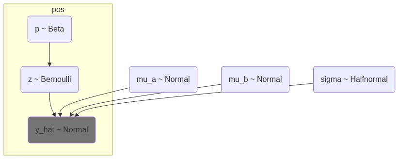
The simplest modeling approach is by regarading each of the bins independent of each other, and to simply draw from one of the distributions based on the encountered E1 value. The probability, \(p\) of being in A is determined using a flat prior, \(Beta(1,1)\), which is assigned to a type, \(z\), with a Bernoulli trial on \(p\). Additionally, the two distributions have a shared standard deviation out of a HalfNormal distribution, \(\sigma \sim \mathcal{HN}(1)\). That is,
where \(y_i\) is the observed E1 value at bin \(i\), \(z_i \in \{0, 1\}\) is the latent compartment assignment (0 = B, 1 = A). 8 chains of 1000 samples (and \(8x1000\) tuning samples) results in 8000 posterior samples after the model has run.
The model might be able to fit well to the observed data, but it is unlikely that it can generalize. Here it is as a Mermaid-js diagram, embedded from the builtin Mermaid-representation of PyMC.
Figure 1: Simple i.i.d. model for E1 values. p is the probability of a bin being in compartment A, z is the latent state variable indicating whether a bin is A or B, and mu_a and mu_b are the expected means for A and B compartments, respectively. The model assumes that the E1 values are normally distributed around these means with a shared standard deviation sigma.
Model 2: Spatially dependent (Random Walk)
To take into account the autocorrelation along the positional axis, I implement a Gaussian Random Walk (GRW) in the logit space of the compartment assignment. That is, the steps between each assignment probability is restricted with a random walk from a bin i to the next bin i+1. In stead of drawing the compartment probability, \(p\), from a flat prior directly, some new variables are introduced. A GRW is effectively the cummulative sum of steps along the positional axis, and can be defined as centered or non-centered [ref]. The centered version is pre-implemented in PyMC as pymc.GaussianRandomWalk [ref], taking a sigma parameter for standard deviation. In the centered GRW the step size and standard deviations are exploring parameter space together and might ot explore it as efficiently or as quickly as a non-centered model that samples the two parameters independently. On the other hand, the non-centered model might interact more with hyperparameters and data. Better results achieved from a non-centered model might indicate that the data is not informative enough for the tighter restrictions on the posterior emposed by the centered model
Centered GRW
The new variables grw_sigma was sampled from a Half-Normal distribution and given to the logit_p that models the GRW with pymc.GaussianRandomWalk. As noted, both variables explore parameter space together. Then, the logits are converted to probabilities, \(p\), by squishing them through a sigmoid, and finally, the compartment is assigned as in the i.i.d. model by a Bernoulli trial.
There are different opinions on when to reparameterize a centered model into a non-centered model [ref], but in my case, PyMC suggested a reparameterization. The idea is to fit the parameters independently and thus achieve a less restricted exploration of parameter space. In this case, the random walk is modeled as follows: the step size is a separate variable, eps, drawing from a standard Gaussian distribution. Then, the step size is scaled by grw_scale which is drawn from a HalfNormal when adding the each step to the random walk by cummulative summation. Again, the walk is constructed in logit space, \(\mathrm{logit}_w\), and forced through a sigmoid to obtain assignment probabilities, and finally, the assignment is performed with a Bernoulli trial on \(w\):
To be able to comparatively evaluate the models, we must establish exactly what we are modeling. The biological assumptions we make is that 1) a given genomic region can be one type at a time, and 2) the autocorrelation between intervals along the genome can be modeled by probabilistic smoothing of the E1 track, even at 10kb resolution. The goal is not to discover new compartments, but to model the transitions between compartments with the assumption that some peaks or dips in E1 that barely causes a sign change are potentially caused by noise and are thus not of biological relevance. Of course, the ability to model this behaviour relies heavily on the assumption that the value of the E1 track carries information about the distinction between compartments additional to that of the sign of the vector.
In a classical setting, the way to compare Bayesian models is by some measure of how much information a model has learned from the data it was trained on. Arviz provides the Akaike Information Criterion (AIC) and the Widely Applicable Information Criterion (WAIC), where it uses leave-one-out cross-validation to generate the out-of-sample predictive accuracy. Conveniently, the arviz.compare takes multiple models and generates a neat table with the results of its cross-validation analysis.
However, when an expected result of the model is that some peaks or small compartments are reduced or smoothed, we must question the interpretability of these criteria. At least, the balance between generalization and fitting should be skewed towards generalization, expectedly at the cost of fitting.
Results
The Eigendecomposition
Discussion
The discussion
Conclusion
I am concluding this analysis
Bon mot
Nothing in Biology Makes Sense except in the Light of Evolution
- Theodosius Dobzhansky
References
Abril-Pla, Oriol, Virgile Andreani, Colin Carroll, Larry Dong, Christopher J. Fonnesbeck, Maxim Kochurov, Ravin Kumar, et al. 2023. “PyMC: A Modern, and Comprehensive Probabilistic Programming Framework in Python.”PeerJ Computer Science 9 (September): e1516. https://doi.org/10.7717/peerj-cs.1516.
Lajoie, Bryan R., Job Dekker, and Noam Kaplan. 2015. “The Hitchhiker’s Guide to Hi-C Analysis: Practical Guidelines.”Methods (San Diego, Calif.) 72 (January): 65–75. https://doi.org/10.1016/j.ymeth.2014.10.031.
Lieberman-Aiden, Erez, Nynke L. Van Berkum, Louise Williams, Maxim Imakaev, Tobias Ragoczy, Agnes Telling, Ido Amit, et al. 2009. “Comprehensive Mapping of Long-Range Interactions Reveals Folding Principles of the Human Genome.”Science 326 (5950): 289–93. https://doi.org/10.1126/science.1181369.
Wang, Yao, Hanben Wang, Yu Zhang, Zhenhai Du, Wei Si, Suixing Fan, Dongdong Qin, et al. 2019. “Reprogramming of Meiotic Chromatin Architecture During Spermatogenesis.”Molecular Cell 73 (3): 547–561.e6. https://doi.org/10.1016/j.molcel.2018.11.019.