Introduction
The X chromosome plays a unique role in evolution, being directly exposed to selection pressures due to its hemizygosity in males, leading to unique inheritance patterns. Regions of reduced diversity on the X chromosome could reflect the influence of strong evolutionary forces that are aided by structural features of the genome. Chromatin architecture, particularly the organization into A/B compartments, may provide insights into the functional basis of these patterns.
Here, I analyze the 3D chromatin structure of the X chromosome in rhesus macaque (Macaca mulata) using Hi-C data on the latest reference genome (rheMac10). The analysis extensively combines software tools that emphasize reproducibility, ensuring that the analyses are transparent, portable, and replicable.
Evolution on X
The production of gametes in a sexually reproducing organism is a highly complex process that involves numeruous elements. Spermatogenesis, the process of forming male gametes, involves four stages of differentiation from a germ cell through spermatogonia, pachytene spermatocyte, and round spermatids to spermatozoa (Wang et al. 2019), and is the basis of male reproduction. The specialized cell division of meiosis neatly handles the pairing, recombination, and segregation of homologous chromosomes, thereby ensuring proper genetic distribution. A thorough understanding of the molecular steps of reproduction and how genetic material is inherited is essential in biology, bringing insight to areas such as speciation, population diversity, and infertility.
Sex chromosomes differ from autosomes in several ways, primarily due to their unique inheritance patterns and copy number. The Y chromosome is present only in males, with a single copy per individual. The X chromosome, on the other hand, has a more complex inheritance pattern: males have one copy, while females have two. As a result, X chromosomes spend two-thirds of their time in females and only one-third in males. This skewed ratio influences the dynamics of selection on the X chromosome. Furthermore, in males, the single-copy nature of the X chromosome (hemizygosity) means that any mutations or loss of function are directly exposed, as there is no second copy to compensate. This concept also underpins Haldane’s rule (Haldane 1922), which states that in hybrids of two species, the heterogametic sex (e.g., XY in mammals, ZW in birds) is the first to exhibit reduced fitness, such as sterility, or to disappear entirely. Even a century later, the exact reasons for this phenomenon remain debated, with several hypotheses proposed. These include:
- Y-incompatibility: The Y chromosome must remain compatible with the X chromosome or autosomes.
- Dosage compensation: Hybridization may disrupt crucial dosage compensation mechanisms in heterogametic individuals.
- Dominance: Recessive deleterious alleles may cause sterility when expressed in the heterogametic sex.
- Faster-male evolution: Male reproductive genes may evolve more rapidly than female ones, leading to incompatibilities.
- Faster-X evolution: X-linked loci may diverge more quickly than autosomal loci, contributing to hybrid sterility.
- Meiotic drive: Conflicts between drivers and suppressors on sex chromosomes may result in sterility.
These hypotheses highlight the intricate interplay between sex chromosomes, selection, and hybridization (Cowell 2023). Furthermore, although this phenomenon is observed across various taxa and even kingdoms, the underlying explanations differ, and there is no universal consensus for all species. In many cases, multiple mechanisms from the listed explanations are thought to act in concert (Lindholm et al. 2016). The complexity of selection on the X chromosome remains an area of active research, with numerous studies suggesting strong selection pressures on the X chromosome across primates. This topic is explored in greater detail in the following sections.
Extended Common Haplotypes (ECH) on human X
Incomplete lineage sorting (ILS) occur when all lineages in a population are not completely sorted between two speciation events, resulting in a gene tree incongruent with the species tree (Mailund, Munch, and Schierup 2014). Briefly, it complicates phylogenetic inference as it implies that divergence time does represent speciation time. But, by solving the incongruency with a maximum likelihood approach (see Mailund, Munch, and Schierup 2014), the relation between the ILS proportion, \(p\), time between two speciation events, \(\Delta\tau\), and effective population size, \(N_e\), is given by the formula
\[ N_e = \frac{\Delta\tau}{2} \ln \frac{2p}{3}. \]
Then, by comparing the observed (local) ILS with the expected (e.g. a genomic average), a reduction in \(N_e\) can be used to infer selection. Additionally, as selective sweeps force lineages to coalesce, sweeps will also cause a reduction in ILS. Dutheil et al. (2015) found that the human X chromosome had reduced ILS compared to autosomes on a third of its sequence, fully explaining the low divergence between human and chimpanzees. Reduced ILS co-occur with reduced diversity across the X chromosomes of great apes, including human. Additionally, Neanderthal introgression was depleted in the same regions, and the authors suggest that they are a target of selection, as they rule background selection to be responsible for reduced ILS.
Low-diversity regions on the human X chromosome that also overlap with reduced human-chimp ILS have been hypothesized to arise from selective sweeps between 55,000 (archaic introgression after out-of-Africa event) to 45,000 (Ust’-Ishim man) years ago (Skov et al. 2023). The authors define the time-span by comparing haplotypes of unadmixed African genomes with admixed non-African genomes. Here, they locate megabase-spanning regions on the X chromosome where a large proportion of the non-African population have reduced archaic introgression, hypothesizing that selective sweeps have created these extended common haplotypes (ECHs). The ECHs span 11% of the X chromosome and are shared across all non-African populations. Similar to the low-ILS regions, ECHs exhibit a complete absence of archaic introgression (Neanderthal and Denisovan). Notably, the largest continuous ECH spans 1.8 Mb—more than double the size of the selective sweep associated with the lactase persistence gene, which represents strongest selective sweeps documented in humans (Skov et al. 2023; Bersaglieri et al. 2004). If such strong selection underlies the observed low diversity, it suggests that factors beyond fitness effects alone may be contributing to this pattern. This raises the possibility that the observed patterns of low diversity may result not only from strong selective sweeps but also from several factors in combination. Structural elements, such as physical linkage between the regions within ECHs, may facilitate coordinated selection, maintaining reduced diversity over extended genomic stretches. Additionally, sex-specific pressures, such as those linked to the unique transmission and evolutionary dynamics of the X chromosome, could contribute to this pattern. Further investigation is needed to disentangle the roles of these mechanisms in shaping the genomic landscape of the X chromosome.
Disproportionate minor parent ancestry on baboon X
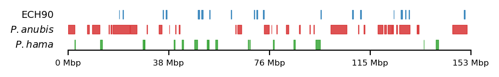
As mentioned above, low ILS and reduced diversity is consistent across all great apes, and thus the regions have been investigated in baboons as well. Sørensen et al. (2023) have mapped the interspecies gene flow between baboon genomes in their evolutionary history, which revealed male-driven admixture patterns in six different baboon species. The authors infer a male-driven admixture from mismatching phylogenies of the mitochondrial DNA and the nuclear DNA. This indicates a role of nuclear swamping, where the nuclear DNA from one species progressively replaces that of another through repeated hybridization and backcrossing, while the mitochondrial DNA, inherited maternally, remains unaffected. This pattern suggests that male-driven gene flow plays a significant role in shaping the genomic landscape of these regions, potentially impacting diversity and co-ancestry across species. Sørensen et al. (2023) compare the ratio of admixture between chromosome 8/X across the populations, which support the same pattern. Recently, in a yet unpublished analysis by Munch (2024), exceptionally large regions (up to 6 Mb, averaging 1 Mb) were identified on X in olive baboon (Papio anubis), where either all individuals had olive ancestry, or 95% of the individuals had hamadryas ancestry, significantly diverging from the background proportions, suggesting that these regions may be under strong selective pressures, are influenced by structural genomic features that limit recombination, or potentially both. Such patterns suggest that certain chromosomal regions are either preserved due to adaptive advantages or subjected to sex-biased gene flow, further reinforcing the impact of male-driven admixture on shaping genomic variation. These findings highlight the complexity of admixture dynamics and their potential to create localized genomic signatures that deviate from overall ancestry proportions.
Sørensen et al. (2023) highlights the importance of studying these populations, as they serve as models for understanding genomic separation in archaic hominin lineages while inhabiting comparable geographic ranges. Studying closely related, extant primate species provides a unique opportunity to gain insight into how hominin (human, Neanderthal, Denisovan) phylogenies were formed. By analyzing the intricate effects of population structure, migration, and selection in these species, we can draw parallels and infer events in our own archaic evolutionary history. See Figure 1 for a genomic overview of the abovementioned sets of regions.
Chromatin Architecture
The specific regions under strong selection identified across primate species, including humans and baboons, are all located on the X chromosome and span megabase-scale genomic regions. As mentioned above, alternative mechanisms, such as the chromosomal architecture and its rearrangements, could play critical roles in facilitating, regulating, or buffering these regions from selective forces.
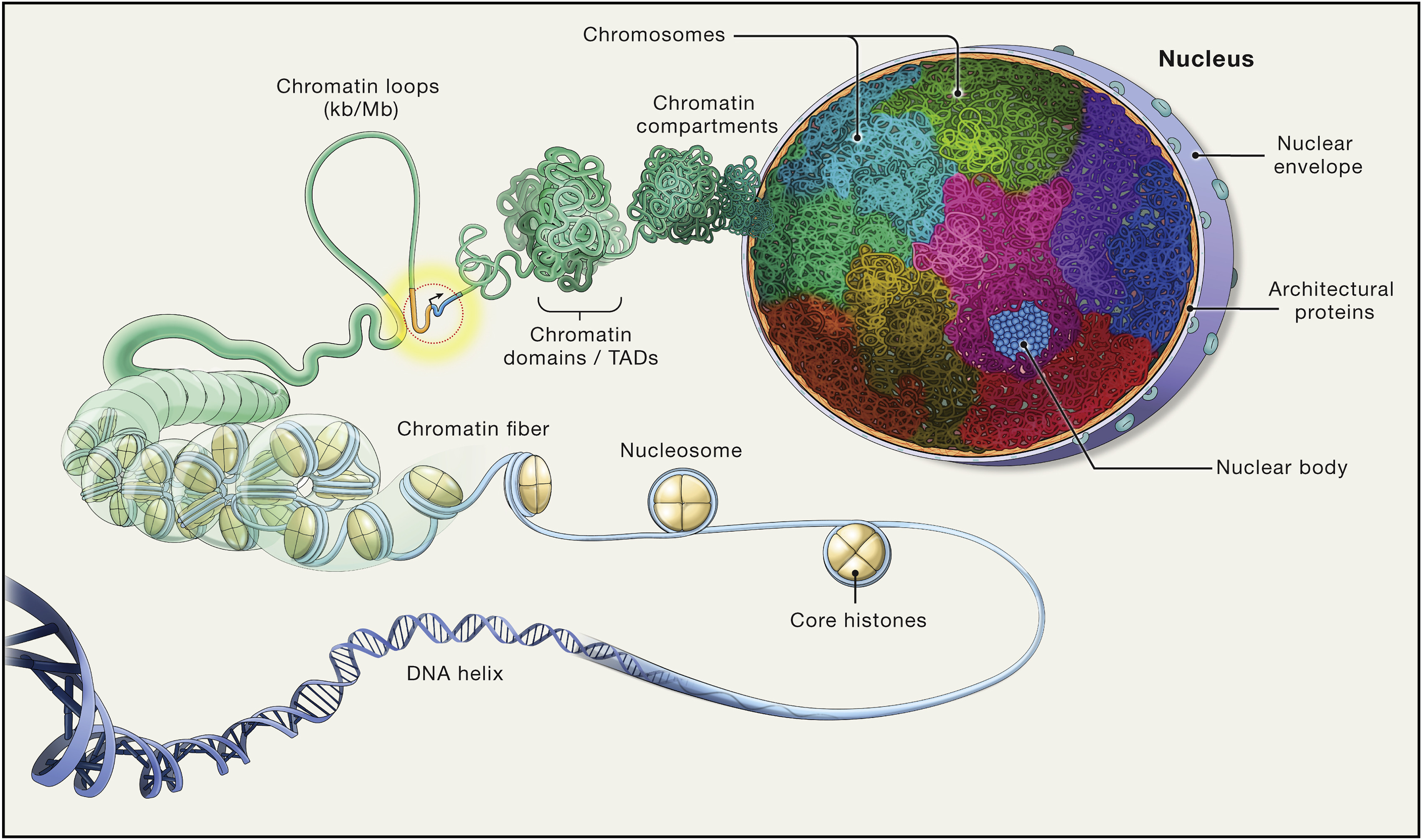
Therefore, understanding the genome organization and variation could gain insights regarding mechanisms of selection as well. Chromatin has long since been implicated in gene regulation and the functional state of the cell (Lieberman-Aiden et al. 2009), as the three-dimensional structure of the chromosome can bring distant regions in close proximity, and disrupting the organization can lead to development abnormalities (Dixon et al. 2015). Chromatin is hierarchically compartmentalized, meaning multiple orders of organizaion can be nested under each other (see Figure 2). At the large end, compartments can span multiple megabases (Lieberman-Aiden et al. 2009), and in the small end as little as 500 base pairs have been showed to aid subgenic structural organization. Even at sub-megabase scales, at the level of topologically associating domains (TADs) or chromatin loops (Ramírez et al. 2018; Zuo et al. 2021), the structure helps segregate regulatory elements and ensure proper function.
Analyzing 3D chromatin data from rhesus macaques, a widely used primate in experimental studies, could answer the question of whether regions under selection are intertwined with chromosomal organizational features. Studying the chromosomal architecture through gametogenesis, particularly spermatogenesis, could provide valuable insights about meiotic recombination and its relationship to genome organization. If they correlate with regions under selection across primates, we have new mystery to explain.
Wang et al. (2019) found that through the stages of spermatogenesis, chromatin compartmentalization undergo massive reprogramming, going from megabase-spanning compartments through smaller, refined compartments and back to the megabase compartments. The reprogramming is conserved between rhesus macaque and mouse, indicating a very important feature of the organization, but the author does not test whether genomic positions of the compartments are conserved between species. Extending their analysis of chromatin compartmentalization through spermatogenesis could make an obvious starting point for investigating the relationship between yet another set of megabase-spanning regions and those of strong selection identified above.
3C: Chromatin Conformation Capture
The first method developed to capture long-range interactions between pairs of loci was 3C, which uses spatially constrained ligation followed by locus-specific PCR (Lieberman-Aiden et al. 2009). Subsequent advancements introduced inverse PCR (4C) and multiplexed ligation-mediated amplification (5C). A limitation common to these methods is their inability to perform genome-wide, unbiased analyses, as they require predefined pairs of target loci.
DNA can be organized into different structural levels. 3C focuses on identifying the higher-order organization within the nucleus, such as when the 30 nm chromatin fiber folds into loops, Topologically Associating Domains (TADs), and chromatin compartments.
Hi-C: High-Throughput 3C
The introduction of the Hi-C (high-throughput 3C) method (Lieberman-Aiden et al. 2009) opened new possibilities for exploring the three-dimensional organization of the genome, as deep-sequencing technologies combined with high-performance computing allow for genome-wide analysis that is unbiased. Lieberman-Aiden et al. (2009) show that when combining spatially constrained ligation with deep parallel sequencing and subsequent analysis, we can infer distinct chromosomal territories as intrachromosomal contacts were significantly less abundant than interchromosomal contacts. The method also confirmed the spatial separation of two chromatin conformations in its active (open) state or inactive (closed) state, as they were significantly correlated with distances measured by fluorescence in-situ hybridisation (FISH). The two comformations were termed A- and B-compartments, respectively, and A defined to positively correlate with gene density. Finally, they showed that loci are physically more proximal when they belong to the same compartment implying that Hi-C reads serves well as a proxy for distance. Later, several smaller-order domains were inferred with the same method, such as topologically associating domains (TADs) and chromatin loops. Here, we narrow our focus on the largest of the structures, compartments, that is known to determine availability to transcription factors, thus making an A compartment active—and the B compartment inactive.
Hi-C Library preparation
A specialized protocol for preparing the DNA library is necessary (Lieberman-Aiden et al. 2009, fig. 1a). Briefly, formaldehyde is used to crosslink spatially adjecent chromatin. Restriction enzyme HindIII is used to digest the crosslinked chromatin, leaving sticky ends, 5-AGCT-3, that are filled and biotinylated with a polymerase (using either biotinylated A, G, C, or T). The strands are ligated in highly dilute conditions, which is favoring the ligation of the two crosslinked strands, forming chimeric, biotinylated strands. Upon ligation, the restriction site is lost as a biotinylated 5-CTAG-3 site (also referred to as the ligation junction) is formed. Lastly, the ligation junctions are isolated with streptavidin beads and sequenced as a paired-end library.
To be able to create stage-resolved Hi-C library of spermatogenetis, several steps have to be performed on the samples before crosslinking. First, the samples have to be treated immediately after harvesting to ensure viable cells. Secondly, the samples have to be purified to accurately represent each stage og spermatogenesis. Specifically, the data for this project (Wang et al. 2019, acc. GSE109344) preluded the library preparation protocol by sedimentation-based cell sorting to separate live spermatogenic cells into different stages of differentiation, namely spermatogonia, pachytene spermatocyte, round spermatid, and spermatozoa. Then, the cells were fixed in their respective state before crosslinking. The authors use their own derived method for library preparation, termed small-scale in-situ Hi-C, allegedly producing a high-quality Hi-C libary from as little as 500 cells (capturing the variance of millions of cells).
Initially, Hi-C library preparation was designed to generate molecules with only a single ligation site in each, but with advancements in sequencing technology (‘short-reads’ can now span several hundreds of base pairs) and the shift to more frequently cutting restriction enzymes for higher resolution results in multiple ligation events per sequenced molecule (Open2C et al. 2024), which is adressed in the section below.
Hi-C Data Analysis
The analysis of the read-pairs of a Hi-C library is divided into several smaller tasks, see Figure 3.
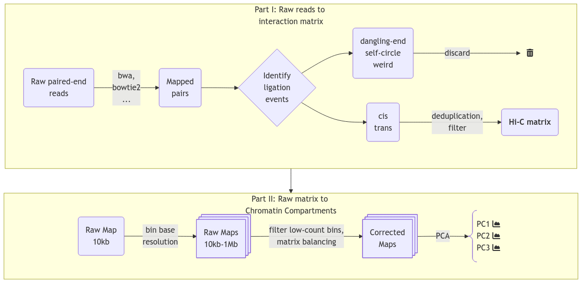
The reads must be aligned to the reference in such a way that the intentional chimeric read-pairs (as per above-mentioned protocol) are rescued, and unintentional read-pairs are discarded. That is, we must make sure they represent ligation junction of adjecent chromatin segments, and not technical artefacts or unintentional (random) fusions of unrelated DNA.
Aligning the Hi-C reads
The main difference between Hi-C libraries and standard paired-end libraries is the high fraction of chimeric reads in Hi-C. As a contact pair is crosslinked and ligated before sequencing, chimeric reads occur as a feature, and standard mapping techniques seeks to filter out this type of reads (Lajoie, Dekker, and Kaplan 2015). Thus, we need specialized tools for rescuing chimeric reads. That said, we have to be cautious distinguishing the intended chimerism for Hi-C and that of technical artefacts. Any software for local alignment can be used for aligning reads from a Hi-C library. However, one should make sure to disable paired-end rescue mode if possible, otherwise each read in a pair (each mate) should be aligned separately (Lajoie, Dekker, and Kaplan 2015). This removes the assumption that the distance between mates fits a known distribution because the genomic sequences originate from a continuous DNA-fragment. For example, the bwa-mem (Li 2013) implementation of this (the -P option) activates the Smith-Waterman algorithm to rescue missing hits, but disables the search of hits that fit a ‘proper’ pair. After alignment, each read is typically assigned to the nearest restriction fragment to enable categorization of pairs into different categories.
Interestingly, this last step is not included by default in pairtools, as Open2C et al. (2024) observe very similar statistical properties on pairs that are either close or distant from the nearest restriction site. Thus, restriction fragment filters are not needed, and instead, a simple filter is applied against short-distance pairs that is automatically calibrated.
Identifying and Storing Valid Hi-C Pairs
One should be cautious when filtering invalid from valid pairs, as they are not easily distinguished. A ligation event will be categorized into one of five categories (see Table 1): dangling-end, self-circle, weird, intrachromosomal (cis), and interchromosomal (trans) (Bicciato and Ferrari 2022, Ch. 1). Either dangling-end or self-circle events are reported if a read-pair maps to the same restriction fragment depending on the orientation, and deemed uninformative (Lajoie, Dekker, and Kaplan 2015). Usually, weird events are demeed uninformative as well, as it is challenging to distinguish a sequencing error from the result of a diploid fragment. PCR duplicates should be discarded as well, having either identical genomic sequence, or sharing exact 5’ alignment positions of the pair (Lajoie, Dekker, and Kaplan 2015; Bicciato and Ferrari 2022, Ch. 1). The probability that such pairs are valid (i.e. there are multiple of the same pairs) is very low. We also have to distinguish between molecules with only a single ligation event (one-way contact) or multiple ligation events (multi-way contacts). For that, a descision should be made on whether to 1) discard molecules with multiple ligations, 2) report one of the ligations (e.g. the 5’-most in both directions), or 3) report all events on a molecule.
| Event name | Explanation |
|---|---|
| Dangling-end | Non-digested collinear fragments. Fraction can be high. |
| Self-circle | Collinear fragment(s) have circularized. Very low fraction could indicate unsuccesful ligation. |
| Weird | Mates have the same orientation on the reference. Is not possible with single copy fragment. Either sequencing errors or diploid fragments1. |
| Cis | Pairs from the same chromosome (intrachromosomal) |
| Trans | Pairs from distinct chromosomes (interchromosomal) |
Quality Control and Interaction Matrices
To determine the quality of the Hi-C library, most tools generate quality control log files at some point during the filtering steps, which can then be aggregated and analyzed (with e.g. MultiQC Ewels et al. (2016)). The ratios between the different ligation events can be informative about the quality of the Hi-C library. Here, both the distribution of discarded reads across categories, as well as the ratios between cis/trans interactions for a certain organism provide information about the library. For example, the biases of different aligners might be captured by comparing the reason why reads are discarded between two different aligners, as well as whether or not there is a preference of cis or trans in an aligner itself. This allows for evaluating the mapping parameters as well as the filters applied downstream. Additionally, \(P(s)\), the contact probability as a function of genomic separation can be inspected as it should decay with increasing distance. The trans/cis-ratio can sometimes be a good indicator of the noise level in the library, and additionally, the level of random ligation events can be quantified by counting the number of trans events occurring to mitochondrial genome. They should not occur naturally, as the mitochondrial genome is separated from the DNA in the nucleus. This method has some pitfalls that should be controlled for; some parts of the mitochondrial genome can be integrated into the host genome, and mitochondrial count may differ between cell-stages.
Typically, a filter against low mapping quality is applied on the data before constructing the interaction matrix (Hi-C matrix), and a conventional threshold is \(mapq < 30\) (Bicciato and Ferrari 2022). However, a considerable amount of reads do not pass that threshold, and thus we risk discarding potential valid information and should make sure to have enough data. Consequently, HicExplorer defaults to a lower threshold (\(mapq < 15\)), and pairtools enforces no filter by default, but recommends setting this manually (starting at \(mapq < 30\)).
A Hi-C interaction matrix simply maps the frequency of interactions between genomic positions in a sample. The maximum resolution of a Hi-C matrix is defined by the restriction enzyme, where the size of the restriction site (probabilistically) determines average space between each cut. With a 4 bp restriction site, the fragments will average \(4^4 = 256 bp\) and similarly \(4^6 = 4096 bp\) for a 6 bp restriction site. This leads to ~12,000,000 and ~800,000 fragments, respectively. Very deep sequencing is required to achieve enough coverage to analyze the interaction matrix at the restriction fragment resolution, but, usually, such high resolution is not required. Therefore, it is common practice to bin the genome into fixed bin sizes, which also enables a more efficient handling of the data if the full resolution is not needed (e.g. when plotting large regions such as a whole chromosome). The conventional format to store a Hi-C matrix, consisting of large multidimensional arrays, is HDF5. Each HDF5 file can store all resolutions and metadata about the sample, resolutions typically ranging from 10kb to 1Mb. Typically, the stored resolutions should be multiples of the chosen base-resolution, as the lower resolutions are constructed by recursive binning of the base resolution. cooler (Abdennur and Mirny 2020) neatly offers efficient storage with sparse, upper-triangle symmetric matrices and naming-conventions of the groups in their .h5-based file format, .cool, and they provide a Python class Cooler as well for efficiently fetching and manipulating the matrices in Python.
Inferring from the matrix (Calling Compartments)
The raw frequency matrices are generally not very informative, as the contact frequencies vary greatly between bins and contain biases in addition to the \(P(s)\) decay, which results in a diagonal-heavy matrix with high amount of noise the further we travel from the diagonal. Therefore, to analyze the three-dimensional structure of the chromatin, a method for correcting (or balancing) the raw Hi-C matrix has to be applied. It is unadvisable to correct low-count bins as it will greatly increase the noise, or to correct very noisy bins, or very high-count bins. Therefore, some bin-level filters are applied before balancing (Lajoie, Dekker, and Kaplan 2015);
- Low-count bins are detected by comparing bin sums to the distribution of bin sums with a percentile cutoff,
- Noisy bins are detected by comparing bin variance to the variance distribution of all bins (and percentile cutoff), and
- Outlier point-interactions are removed (a top-percentile of bin-bin interactions)
Iterative Correction and Eigendecomposition (ICE) (Imakaev et al. 2012) is a widely used method for correcting multiplicative biases in Hi-C data. ICE operates on the assumption that all loci should have roughly equal visibility across the genome, meaning that the total number of interactions per locus should be uniform. It corrects the raw interaction matrix by iteratively scaling rows and columns until they converge to a consistent coverage. By leveraging pairwise and genome-wide interaction data, ICE calculates a set of biases for each locus and normalizes the interaction frequencies accordingly. This process results in a corrected interaction matrix with uniform coverage, smoother transitions, and reduced visibility-related biases. Notably, ICE does not distinguish between different sources of bias, instead calculating a collective bias for each locus. Imakaev et al. (2012) show that known biases are factorizable by comparing their results to predictions of restriction fragment biases, GC content, and mappability from a computationally intensive probabilistic approach. By showing that the product of those known biases explain \(>99.99%\) of the variability in their bias estimation, they argue that both known and unknown biases will be captured with their iterative correction method (also denoted matrix balancing).
Even with a binned, filtered, and balanced matrix, we are still left with the challenge of translating the matrix into biologically relevant inferations. Importantly, we have to remember that the matrix arise from a collection of cells and that the interaction frequency cannot be translated to a fraction of cells. Additionally, the effect from averaging interaction patterns can cause both individual patterns to be burried and the average pattern to show a pattern that does not exist in any of the single cells. Therefore, when pooling matrices one must make sure that the samples are as similar as possible (e.g. the same differentiation stage and so on). We can also not distinguish interactions that either co-occur in the same cell or ones that are mutually exclusive. Lastly, the way interaction patterns are defined poses a challenge; we define the chromatin compartments to be the output of a method, the ‘E’ in ‘ICE’, eigendecomposition, not as a specific pattern that we can explicitly search for. Although experimentally verified to tightly correlate with chromatin states (Lieberman-Aiden et al. 2009), the inferred compartments vary with different methods of calculating the eigenvector, as dicussed in Section 2.3.0.9 and Section 3.2.3. To further complicate the challenge, interaction patterns on different scales co-exist and are difficult to disentangle without simplifying assumptions, such as assuming that small-scale interactions are not visible (or are negligible) at a certain resolution, or restricting the viewframe to eliminate large-scale variance between chromosome arms. It is by definition a speculative exercise to interpret the biological relevance of an observed pattern, but the consensus is to call compartments on interacting regions that arise from the eigendecomposition of a Hi-C matrix without further modifications (Lajoie, Dekker, and Kaplan 2015). Briefly, each genomic bin is assigned a value reflecting its compartment identity, where positive values indicate compartment A and negative values indicate compartment B. The interaction score between two loci is represented as the product of their compartment values, resulting in enriched interactions for loci within the same compartment (positive product) and depleted interactions for loci in different compartments (negative product). This model reproduces the checkerboard pattern characteristic of Hi-C data. Principal component analysis (PCA) identifies the first principal component, which optimally captures the strongest compartment signal. The sign of this component determines whether a locus belongs to compartment A or B. As the eigenvector is only unique up to a sign change, a phasing track is used to orient the eigenvector, aiming for a positive correlation with GC content (in mammals), so that A-compartments represent the active euchromatin, while B-compartments represent the closed heterochromatin.
Compartment Edges and Genomic Intervals
As arbitrarily as a compartment may be defined, we chose to define another genomic interval for analysis. It is well known that CTCF and other structural proteins preferentially binds to Topologically Associating Domains (Bicciato and Ferrari 2022, Ch. 3) (TADs; they were initially defined as sub-Mb chromatin structures (Lajoie, Dekker, and Kaplan 2015), but currently the definition seems to vary based on the method of extraction (Open2C et al. 2022)). Derived from this, we define a transition zone between A/B compartments to look for enrichment of specific regions of interest.
We can test if two sets of genomic intervals correlate (say, compartment edges and ECH regions) by either proximity of the non-intersecting parts of the sets, or by intersection over union (Jaccard index). When the underlying distribution of a statistic (or index) is unknown, a widespread method in statistics for estimating a p-value is by bootstrapping. Here, one of the sets are bootstrapped (the intervals are placed at random positions) a number of times, \(b\), and the fraction of statistics more extreme than the one we observe is reported as the p-value.
Reproducibility Infrastructure
Reproducibility is a cornerstone of the scientific method, ensuring that findings can be independently verified and built upon by others. Without it, the credibility of research findings is undermined, hindering scientific progress by becoming anecdotal. The necessity of reproducibility also aligns with scientific skepticism—the practice of critically evaluating evidence and methods to guard against biases or errors. As research grows increasingly computational, robust reproducibility infrastructure is essential to maintain these principles (Baker 2016), facilitating transparency, validation, and collaboration across diverse scientific disciplines. Thus, apart from the biological questions we seek to investigate and answer in this thesis, a major goal is to create fully (and easily) reproducible results through a self-contained and version-controlled pipeline using git (Torvalds and Hamano 2005), GitHub (GitHub, Inc. n.d.), quarto (Allaire et al. 2024), Anaconda (Anaconda Software Distribution 2016), gwf (GenomeDK 2023), and Jupyter (Kluyver et al. 2016). The result is a fully reproducible analysis, including figures and tables in only 3 lines of code2 (Listing 1) . See Table 2 for a brief overview:
| Tool | Description |
|---|---|
| Jupyter | Interactive coding environment for analysis and development (notebooks are natively rendered with Quarto) |
| Quarto | A Quarto Manuscript project nested inside a Quarto Book for rendering html (website) and PDF (manuscript) from Markdown via Pandoc. Supports direct embedding of output from Jupyter Notebook cells (plots, tables). |
| Conda | For managing software requirements and dependency versions reproducibly. |
| git | Version control and gh-pages branch for automated render of Quarto project |
| GitHub | Action was triggered on push to render the project and host on munch-group.org |
| gwf | Workflow manager to automate the analysis on a HPC cluster, wrapped in Python code. workflow.py currently does everything from .fastq to .cool, but notebooks can be set to run sequentially as part of the workflow as well. |
GWF: workflow management for High-Performance Computing (HPC)
To enable consistently reproducing the analyses, a workflow manager is utilized. Several exist, but the most well-known is likely Snakemake. However, we use the pragmatic (authors’ own words), lightweight workflow manager GWF, which is optimized for the GenomeDK insfrastructure, and has the benefit of in-house support.
Briefly, GWF works on a python script, conventionally workflow.py, that wraps all the jobs (targets in gwf lingo) you will submit to the HPC cluster. Each target is submitted from a template, written as a Python function, which includes inputs and outputs that GWF should look for when building the depency graph, options list of resources that is forwarded to the queueing system (Slurm in our case), and specs, specifying the submission code in Bash as a formatted Python string (meaning we can pass Python variables to the submission code), providing an extremely flexible framework for running large and intensive analyses in a high-performance computing environment.
Project Initialization
gwf
The initialization of the project directory is the basis of reproducibility and transparency, together with workflow.py inhabiting the main directory. Specifically, it includes a subdirectory for (intermediate) files that are produced by the pipeline, steps/. Everything in this directory is reproducible simply by re-running the gwf-workflow. It is thus not tracked by git, as the large files (raw reads, aligned read-pairs, etc.) it contains are already indirectly tracked (workflow.py is tracked). It can be safely deleted if your system administrator tells you to free up disk space, although you would have to run the workflow again to continue the analysis. Several directories are created for files that are not produced by the pipeline, that is, files that the workflow uses, configuration files, figures edited by hand, etc. Ideally, as few files as possible should be outside of steps/, to be as close as possible to an automated analysis.
Jupyter Notebooks
A notebooks/ subdirectory contains Jupyter notebooks that are named chronologically, meaning they operate on data located in either steps/ or generated from a previous notebook. This way, the workflow can also be set up to run the notebooks (in order) to produce the figures, tables, and their captions used in this manuscript.
Quarto
Quarto is an open-source scientific and technical publishing system that uses (pandoc) markdown to create and share production quality output, integrating Jupyter Notebooks with Markdown and LaTeX and enabling embedding content across .ipynb and .qmd. In .qmd, code chunks in several programming languages can be executed and rendered, including Python, R, mermaid (JavaScript-based diagramming). A Quarto project is configured with a YAML configuration file (_quarto.yml) that defines how output is rendered. In this project, we use a nested structure, nesting a Slides project and a Manuscript project inside a Book project. To manage the directory as a Quarto Book project, a quarto configuration file was placed at the base, defining how the Book should be rendered. Additionally, configuration files were placed in slides/ and thesis/, to render them as Quarto Slides and Quarto Manuscript, respectively. This nested structure lets us render different subprojects with different configurations than the main project, for example to generate the manuscript, a single Quarto Markdown file, in both .html and .pdf, and only including embedded outputs from specified cells from notebooks in the parent directory. Although the Quarto framework is extensive, it is still under development and has several drawbacks worth mentioning. First, one can only embed the output of code cells from notebooks, meaning the only way to embed text with a python variable (e.g. you want the manuscript to reflect the actual value of a variable, sample sizes n = [1000, 10000, 100000], and their respective outputs) is by converting a formatted python string into Markdown and send it to the output. Second, embedded figures will be copied as-is in the notebook, and thus cannot be post-processed with size or layout. This makes it impractical to e.g. use the same figures in slides and in the manuscript. Third, when rendering large projects that is tracked by git, some output files (that have to be tracked to publish the website) can exeed GitHub size limits. Especially if rendering in the jats format, producing a MECA Bundle that should be the most flexible way to exchange manuscripts. However, as not applicable to this thesis, the option was simply disabled. Fourth, some functionality relies on external dependencies that cannot be installed on a (linux) remote host (GenomeDK), such as relying on a browser for converting mermaid diagrams into png for the pdf-manuscript.
git and GitHub
To track the project with git and GitHub, the abovementioned structure was initialized as a GitHub repository, including a workflow for GitHub Actions to publish and deploy the website on the gh-pages branch when pushing commits to main. Briefly, it sets up a virtual machine with Quarto and its dependencies, renders the project as specified in the _quarto.yml configuration file(s), and publishes the project on the group website munch-group.org.
Methods
All computations were performed on GenomeDK (GDK), an HPC cluster located on Aarhus Uninversity, and most of the processing of the data was made into a custom GWF workflow, a workflow manager developed at GDK.
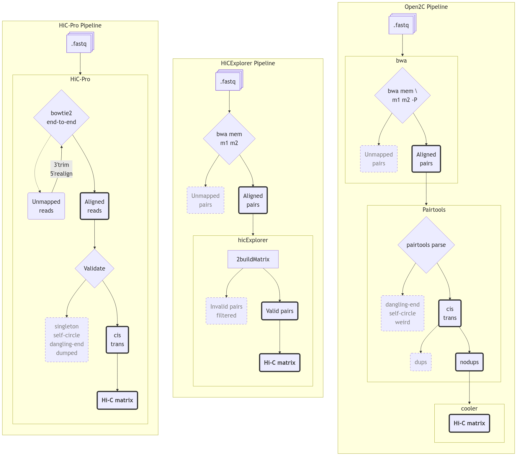
With the analysis tools determined in the above section, I decided it was not feasible to follow the exact approach as Wang et al. (2019) with any of HiCExplorer and Open2C, as they use a third software, HiC-Pro. For mapping the raw reads, Hic-Pro internally uses bowtie2 in end-to-end mode, followed by trimming the 3’-end of the unmapped reads, then remapping the 5’-ends to rescue chimeric fragments. I initially mapped the reads using end-to-end Bowtie2 without the rescue-remapping feature, resulting in a very high fraction of discarded reads. Manually implementing the remapping approach would be impractical. When reanalyzing data, it is important to use state-of-the-art tools. Considering the release timeline (e.g., HiC-Pro v3.1.0 in 2021), both HiCExplorer and Open2C are more recent and likely offer better support for current methodologies. Additionally, the HiC-Pro pipeline stops at a normalized contact map, and is thus not sufficient for downstream analysis. In hindsight, it would have been more sensical to use HiC-Pro to get normalized contact maps, then continue analyzing with cooler/cooltools, and finally compare the results evenly with the results achieved from using Open2C from start to finish. Figure 4 gives an overview of the 3 pipelines metioned in this report.
Fetching raw data
To reproduce the results from Wang et al. (2019), I chose to use their raw data directly from the SRA portal (Sayers et al. 2022). I filtered the data to contain all their paired-end Hi-C reads, and included only macaque samples. The dataset also contains RNAseq data, and the same tissues for both macaque and mouse. The metadata for the dataset was extracted into a runtable SRA-runtable.tsv. To get an overview of the data accessions used in this analysis, we will first summarize the runtable that contains the accession numbers and some metadata for each sample (Table 3). It adds up to ~1Tb of compressed fastq files, holding ~9.5 billion reads, roughly evenly spread on the 5 tissue types.
Fetching and indexing the reference
Wang et al. (2019) use the 2006-version of the macaque reference, rheMac2. Supporting my previous sentiment about not using outdated resources I find it most reasonable to use the latest reference, rheMac10, where Warren et al. (2020) have improved contiguity from rhemac8 by 120 fold, going from N50 contig size of 107 Kbp to 46 Mbp. Reproducing the analysis on the latest assembly of the macaque genome should therefore gain a more accurate read mapping, and consequently a better inference of the chromatin compartments. Therefore, rheMac10 was downloaded to GDK from UCSC web servers. To use bwa for mapping, rheMac10 needs to be indexed with both bwa-index with the --bwtsw option and samtools-faidx, which results in six indexing files for bwa-mem to use. Both bwa-mem and bowtie2 were used in different configurations, and bowtie2 requires its own indexing of the reference, using bowtie2-build with the --large-index option, which creates six index files for bowtie2 to use. The options --bwtsw and --large-index create the special indexing format required for large genomes such as macaque. As we use the position of the centromere to partition chrX into its two arms, and no comment about it was made by Warren et al. (2020), the centromeric region was inferred (visually) from the UCSC browser view of rheMac10, where a large continuous region (chrX:57.5Mb-60.2Mb) had no annotation and showed many repeating regions. The region is roughly the same region as inferred by Wang et al. (2019) by the same method.
HiCExplorer trials
To get aligned reads in a format compatible with HiCExplorer, the read mates have to be mapped individually to the reference genome. This supports the old convention to avoid the common heuristics of local aligners used for regular paired-end sequencing libraries (Lajoie, Dekker, and Kaplan (2015)). HiCExplorer provide examples for both bwa and bowtie2, so I used both with recommended settings. In both cases, the aligner outputs a .bam-file for each mate (sample_R1.bam and sample_R2.bam), and HiCExplorer performs the parsing, deduplication, and filtering of the reads and builds the raw interaction matrix in a single command,
hicBuildMatrix -s sample_R1.bam sample_R2.bam -o matrix.h5 [...]Figure 3 (middle) shows an overview of the pipeline. For parsing, the command needs a --restrictionCutFile, locating the restriction sites from the restriction enzyme used on the reference genome, which is generated with hicFindRestSites that operates on the reference genome and restriction sequence. The default filter, --minMappingQuality 15, was applied as described in Section 1.4.2.3. Notably, HiCExplorer has no options on handling multiple ligations, and the method is undocumented. I assume that Ramírez et al. (2018) have implemented a conservative handling (masking all multiple ligations), as that would have the least consequence.
For the initial exploration of methods with HiCExplorer, I chose five fibroblast samples (see Table 4). The goal was to replicate some of the figures from Wang et al. (2019) using HiCExplorer, especially to reconstruct interaction matrices and E1 graphs from macaque data. We constructed matrices with hicBuildMatrix as described from the separately mapped read-pairs. Along with the matrix .h5 file, a .log file was created as well, documenting the quality control for the sample. Multiple logs were aggregated and visualized with hicQC.
Before correction (or balancing) of the interaction matrix, a pre-correction filter is applied, filtering out low-count bins and very high-count bins. A threshold for Mean Absolute Deviation (MAD) is estimated by hicCorrect diagnostic_plot, followed by iterative correction with hicCorrect correct --correctionMethod ICE. The PCA was performed with hicPCA on the corrected matrices, yielding the first 3 PCs.
The matrix plotting function, hicPlotMatrix, plots matrices directly to .png, and so there is no output sent to the Jupyter display. As I kept the analysis in a Jupyter Notebook (using the buikt-in shell-escape commands to execute bash code), the plot files must be embedded back into the notebook. The command-line options for modifying plots are quite limited, such as adding spacing for a bigWig track with E1 values, including plot titles, or defining the size and resolution of the plot. I made a brief attempt to implement a custom plotting function for the .h5 matrices and bigWig tracks. However, this approach had a major limitation: it could not fetch specific regions from the matrix dynamically and instead required loading entire matrices into memory, including full-length chromosomes.
Open2C pipeline
A GWF workflow was created to handle the first part of the data processing, and each accesion number (read pair, mate pair) from the Hi-C sequencing was processed in parallel, so their execution was independent from each other. See Figure 3 (right) for an overview of the initial steps.
Downloading the reads
The reads were downloaded from NCBI SRA with SRA-toolkit (DevTeam 2024) directly to GDK using the docker image wwydmanski/sra-downloader as gunzipped .fastq files. Although possible to provide a list of accessions to the toolkit, I submitted each accession as a separate target, as SRA-Toolkit acts sequentially, and only starts the next download after all compression tasks were done. It was therefore a low-hanging fruit to parallelize the download for efficiency.
Mapping Hi-C reads
Suspiciously, (“Open2C” n.d.) do not mention any problems with aligning the Hi-C reads, they just provide an example using bwa-mem in paired-end mode and with the -P option set, which activates the Smith-Waterman (Li 2013) algorithm to rescue missing hits, by focusing on assigning only one of the mates to a good mapping and escape mate-rescue. The documentation of bwa state that both bwa-mem and bwa-sw will rescue chimeric reads. Consequently, Open2C does not have a buikt-in way of pairing the reads after mapping, and the reads were thus mapped using Open2C’s recommendations, using their established pipeline for producing a cooler. I chose the latter, where I mapped the fastq files to rheMac10 in paired end mode for a pair (\(m1\), \(m2\)) with bwa mem -SP rheMac10 m1 m2.
Parse and sort the reads
We need to convert the alignments into ligation events, and distinguish between several types of ligation events. The simplest event is when each side only maps to one unique segment in the genome ‘UU’. Other events, where one or both sides map to multiple segments or the reads are long enough (\(>150bp\)) to contain two alignments (multiple ligations) have to be considered as well. Multiple ligations are called walks by Open2C, and are treated according to the --walks-policy when parsing the alignments into valid pairs (or valid Hi-C contacts). Here, mask is the most conservative and masks all complex walks, whereas 5unique and 3unique reports the 5’-most or 3’-most unique alignment on each side, respectively, and all reports all the alignments. The pairs are piped directly into pairtools sort after parsing, as the deduplication step requires a sorted set of pairs. The .pairs-format produced by pairtools is an extension the 4DN Consortium-specified format, storing Hi-C pairs as in Table 5.
| Index | Name | Description |
|---|---|---|
| 1 | read_id | the ID of the read as defined in fastq files |
| 2 | chrom1 | the chromosome of the alignment on side 1 |
| 3 | pos1 | the 1-based genomic position of the outer-most (5’) mapped bp on side 1 |
| 4 | chrom2 | the chromosome of the alignment on side 2 |
| 5 | pos2 | the 1-based genomic position of the outer-most (5’) mapped bp on side 2 |
| 6 | strand1 | the strand of the alignment on side 1 |
| 7 | strand2 | the strand of the alignment on side 2 |
| 8 | pair_type | the type of a Hi-C pair |
| 9 | mapq1 | mapq of the first mate |
| 10 | mapq2 | mapq of the second mate |
I initially used --walks-policy mask, and later followed the recommendations from pairtools, specifically informing that longer reads (\(>150bp\)) might have a significant proportion of reads that contain complex walks. With this in mind and as the average read-length of our data is 300 bp, I decided to re-parse the alignments into a new set of pairs, and equally apply the recommended filter (next section). As both results are saved, we can compare the two approaches.
Filter and deduplicate pairs
Pairtools comes with a de-duplication function, dedup, to detect PCR duplication artefacts. At this point I removed all reads that mapped to an unplaced scaffold. Even though rhemac10 is less fragmented than rhemac8 , rheMac10 still contains more than 2,500 unplaced scaffolds, which are all uninformative when calculating the chromatin compartments as is the goal of this analysis. Therefore, we simply only include the list of conventional chromosomes (1..22, X, Y) when doing the deduplication. Initially, the default values were used to remove duplicates, where pairs with both sides mapped within 3 base pairs from each other are considered duplicates. cooler recommend to store the most comprehensive and unfiltered list of pairs, and then applying a filter it on the fly by piping from pairtools select. The first run that was parsed with mask was not filtered for mapping quality. After reparsing the alignments and applying the same analysis, we compare the two pipelines. A quality control report is generated by pairtools dedup as well, and the reports are merged and visualized with MultiQC (Ewels et al. 2016) for each cell type.
Create interaction matrices (coolers)
The final part of the GWF workflow takes .pairs as input and outputs a .cool file (a cooler). Initially, I read directly from the newly generated deduplicated pairs without additional filtering, but the official recommendation is to filter out everything below \(mapq = 30\) by piping the pairs through pairtools select "(mapq1>=30) and (mapq2>=30)" to cooler cload pairs. I re-parsed the alignments and created new coolers, including only the Hi-C contacts where \(mapq \leq 30\), following the current recommendations from Open2C.
Pooling samples (Merging coolers)
The samples are grouped into replicates with a unique BioSample ID, and I chose to pool all the interaction matrices for each cell type. Even though it is slightly unclear how their replicates are defined, Wang et al. (2019) determine compartments to be highly reproducible between replicates, and they are pooling the replicates as well.
cooler merge was used to merge all samples in each cell-type directory to just one interaction matrix for each cell type. The function merges matrices of the same dimensions by simply adding the interaction frequencies of each genomic position together, resulting in less empty or low-count bins.
Create multi-resolution coolers (zoomify)
A feature of working inside the ecosystem of Open2C is that it natively provides support for storing sparse interaction matrices in multiple resolutions in the same file by adding HDF5-groups to the (multires-)cooler. We can then efficiently store resolutions (i.e., different bin sizes) that is multiples of the smallest bin size. We chose to use 10kb, 50kb, 100kb, and 500kb bins, and the resolutions are made by recursively binning the base resolution. Abdennur and Mirny (2020) call this process zoomifying, and cooler zoomify does the job (it recursively calls cooler coarsen to merge bins).
Matrix balancing (Iterative correction)
Finally, we balance (or correct) the matrices using the cooler CLI. We use cooler balance with the default options which iteratively balances the matrix (Iterative Correction).
We balance the matrices on each resolution, and thus it cannot be done prior to zoomifying. Abdennur and Mirny (2020) state that the balancing weights are resolution-specific and will no longer retain its biological meaning when binned with other weights. Therefore, we apply cooler balance to each resolution separately. cooler balance will create a new column in the bins group of each cooler, weight, which can then be included or not in the downstream analysis. This means we will have access to both the balanced and the unbalanced matrix.
The default mode uses genome-wide data to calculate the weights for each bin. It would maybe be more suitable to calculate the weights for cis contacts only, and that is possible through the --cis-only flag, and that can be added to another column, so that we can compare the difference between the two methods easily. However, when adding the option, the process seemed to stall and had to be terminated manually, and it was not investigated further.
Eigendecomposition
The eigendecomposition of a Hi-C interaction matrix is performed in multiple steps. As value of the eigenvector is only significant up to a sign, it is convention to use GC content as a phasing track to orient the vector. E1 is defined to be positively correlated with GC content, meaning a positive E1 value signifies an active chromatin state, which we denote a A-type compartment (or simply A-compartment). We performed eigendecomposition of two resolutions, 100 kbp and 500 kbp. Wang et al. (2019) briefly describes their method to calculate the eigenvectors as a sliding window approach on the observed/expected matrix in 100 kb resolution summing over 400 kb bins with 100 kb step size, a method I was not able to replicate in the Open2C ecosystem. I decided to mimic this by smoothing the 100 kb E1 values by summing to 500 kb bins in steps of 100 kb, yielding a comparable resolution which I denote ‘pseudo-500 kb’ resolution (ps500kb).
First, we calculate the GC content of each bin of the reference genome, rheMac10, which is binned to the resolution of the Hi-C matrix we are handling. It is done with bioframe.frac_gc (Open2C). To calculate the E1 compartments, we use only within-chromosome contacts (cis), as we are not interested in the genome-wide contacts. cooltools.eigs_cis will decorrelate the contact-frequency by distance before performing the eigendecomposition. eigs_cis needs a viewframe (view) to calculate E1 values, the simplest view being the full chromosome. However, when there is more variance between chromosome arms than within arms, the sign of the first eigenvector will be determined largely by the chromosome arm it sits on, and not by the chromatin compartments. To mitigate this, we apply a chromosome-arm-partitioned view of the chromosome.
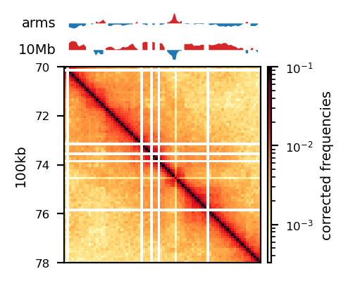
Additionally, to mimic the Local PCA from (Wang et al. 2019), I also defined a view of 10 Mb bins. Thoughout the project, I will compare results from each of the three views and resolutions, and they will be referred to as ‘full’, ‘arms’, and ‘10Mb’ views.
Plotting matrices
We use matplotlib (Team 2024) and seaborn (Waskom 2021) to plot in the Open2C framework. Utilizing the Cooler class, we can fetch regions of the matrix without modifying the file. As my analysis is centered around the X chromosome, it is efficiently handled by simply fetching ‘chrX’ from the matrix with cooler.Cooler.matrix().fetch('chrX'). Many methods of the cooler class returns data selectors, which do not retrieve data before it is queried (Abdennur and Mirny 2020). This means we can create many selectors at once without overflowing memory, enabling us to plot multiple interaction matrices side-by-side, e.g. the corrected and un-corrected matrices. This is easily done with the balance parameter of the matrix selector (.matrix()), which determines if it should apply the balancing weights to the coordinates and defaults to True.
The matrix is retrieved and plotted with matplotlib.pyplot.matshow, which automatically produces a heatmap image of the matrix. Here, instead of transforming the interaction matrix, the color scale is log-transformed with matplotlib.colors.LogNorm. Additionally, cooltools comes with more tools to aid visualization: adative coarsegrain and interpolation, which can be chained. adaptive_coarsegrain iteratively coarsens an array to the nearest power of two and refines it back to the original resolution, replacing low-count pixels with NaN-aware averages to ensure no zeros in the output, unless there are very large regions that exceed the max_levels threshold, such as the peri-centromeric region.
I implemented a plotting utility, plot_for_quarto in notebook 07_various_plotting.ipynb that is compatible with the YAML cell-options read by Quarto’s embed shortcode. It will take an arbitrary number of samples and plot a chromosome (or region) with or without its respective E1 value for either of the three viewframes which has been created. The input is a (subsetted) pandas DataFrame, defined from a file search matching a pattern specified to the glob Python module.
Genomic Intervals
Full Regions, Edges, and Limits
From the eigenvectors, the A-compartments were extracted in bedgraph-format (['chrom', 'start', 'end']) and compared with ECH90 regions lifted to rheMac10 from human. We perform visual inspection of the genomic intervals and test whether ECH90 regions are enriched near the edges of the compartments by defining a 200 kilobase transition-zone centered at each sign change of E1 (referred to as compartment edge). We compare genomic intervals (or sets) both visually by plotting the regions, and by a proximity test and bootstrapping the Jaccard index. Additionally, the compartment limits were invetigated (only 1 flanking base pair) in the same manner. Additionally, the limits were extracted from the baboon datasets and lifted to rheMac10 for comparison.
Proximity test
Determines whether the non-overlapping segments of the sets are more proximal than expected by chance. We define the annotation set and the query set, and the distance from each interval on the query to the most proximal interval on the annotation is used to generate an index of proximity by the mean distance to nearest interval in the annotation. Then, bootstrapping (\(b = 100000\)) is performed by randomly placing the query intervals to generate the null distribution, and finally, the fraction of the null as extreme or more extreme as our observed proximity is reported as the p-value.
Jaccard test
Measures the significance of the observed Jaccard index (intersection over union) between two sets. The index is a measure of similarity (\(intersection/union\)) between two sets (between 0 and 1), which is very sensitive to the size difference between the sets, as even when comparing a set of intervals to a small subset of itself will yield a very small Jaccard index. When we use bootstrapping to generate a null distribution (shuffling the intervals of the query), we find the probability that the two sets (with their respective number and size of intervals), are as similar or more than what we observe. The ratio is reported as the p-value. However, this approach is still sensitive to flipping of query/annotation (if the regions are not the same size), as only the query is bootstrapped.
Multiple testing
Considerations were made to avoid multiple testing biases (p-hacking): Performing tests on all combinations of variables (cell type, resolution, viewframe, query) will yield 90 p-values for each test, and we would have to adjust the significance threshold (with \(\alpha = 0.05\), we expect 4 tests passing the threshold by chance). However, I will narrow down the parameter space based on visualizations and reasoning, leaving fewer combinations to test. I do not find it necessary to correct the conventional significance threshold, \(\alpha=0.05\).
Results
HicExplorer Trials
Quality Control
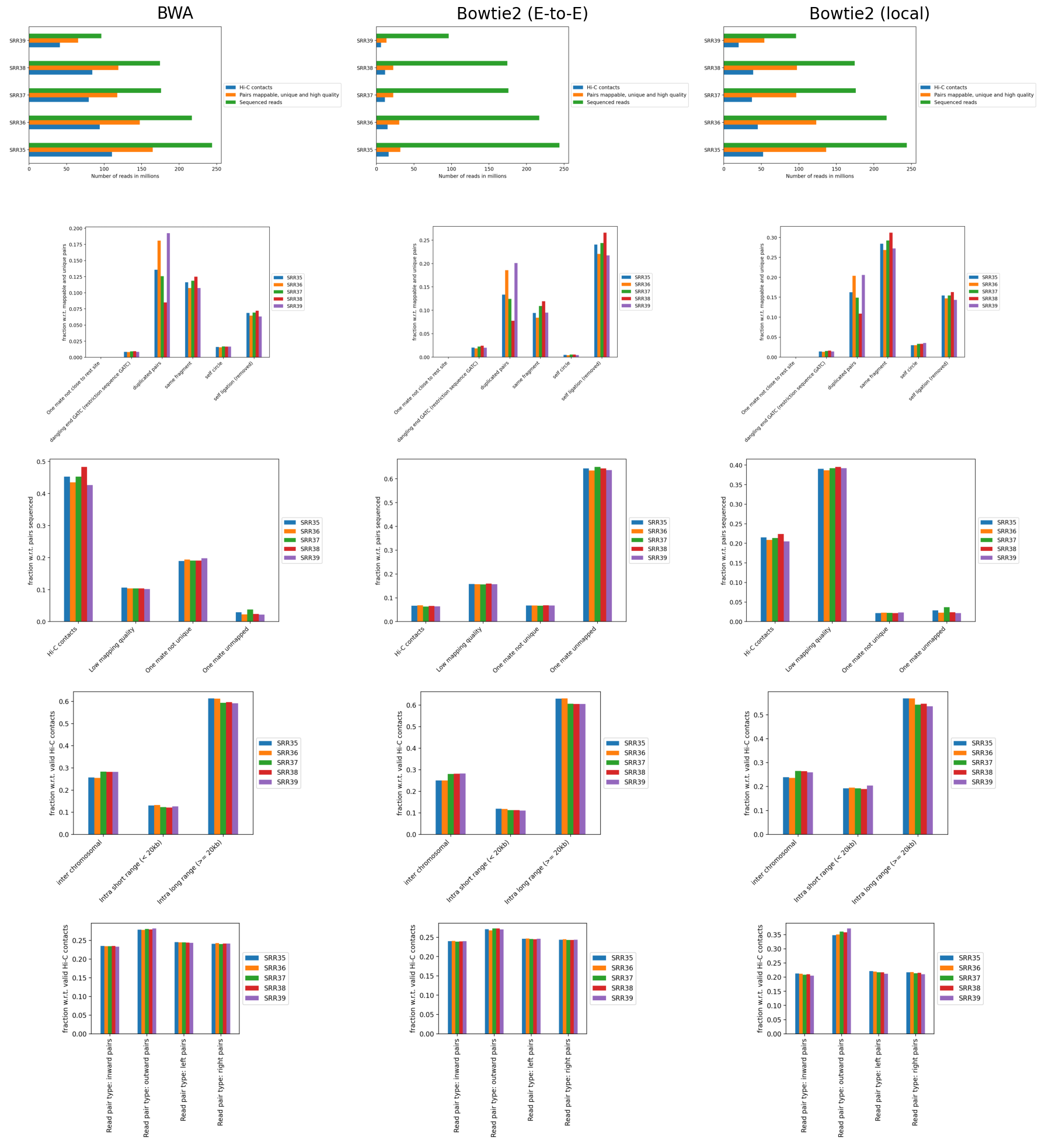
The separately mapped read-mates were parsed into a .h5 interaction matrix by hicBuildMatrix, which include a .log file documenting the buikt-in quality control (hereafter, QC). Log files from the 5 samples were merged with hicQC (Figure 5). I observe equal fractions of the read-orientation of read-pairs (Figure 5, left, row 5), which is expected for a good Hi-C library. Additionally, it determines between 40% to 50% of the total reads to be valid Hi-C contacts (Figure 5, left, row 1), which is usually only 25%-40% (as described in HiCExplorer docs). Figure 5 (left, row 4) shows, however, unusually high fractions of inter-chromosomal contacts (up to 30%) compared to intra-chromosomal contacts (also denoted trans and cis contacts, respectively). It is expected that cis contacts are orders of magnitude more frequent than trans contacts (Bicciato and Ferrari 2022, 2301:236; Lieberman-Aiden et al. 2009), and HiCExplorer states it is usually below 10% for a high-quality library. The high fraction may be mitigated by enforcing a stricter mapq threshold for a valid Hi-C pair, as we also observe higher-than expected valid contacts. However, we continue with the current matrices.
To compare how well these mappings perform, the plotting QC results is an easy way. Therefore, the reads were mapped with bowtie2 in both end-to-end- and local-mode followed by hiCBuildMatrix, and the QC from each method was plotted next to each other (Figure 5). Interestingly, bowtie2 was much more computer-intensive in both modes, perhaps because of the --very-sensitive option. In any case, the QC reveals a major difference in the total number of reads that are determined to be valid Hi-C contacts by hicBuildMatrix. As expected, mapping with end-to-end-bowtie2 makes locating Hi-C contacts more difficult than the other methods (Figure 5, row 1), finding a very low amount of mappable, unique pairs passing the quality threshold. In contrast, mapping with local-bowtie2 performs similarly to bwa in finding mappable, unique, high-quality pairs, but calls only approximately half the number of valid Hi-C contacts (>20%), resulting in a fraction of valid Hi-C pairs that hits the expectation from HicExplorer docs (row3). With bwa, the reads were discarded either due to low mapping quality or non-unique mates, whereas with local-bowtie2, the reads were almost exclusively filtered out due to low mapping quality. This must be a result of how the mappers assign mapping quality, and I believe local-bowtie2 looks suspiciously selective in finding unique but low quality alignments. end-to-end-bowtie almost exclusively filters out read-pairs where one mate is unmapped, which is expected when the majority of reads are unmapped.
hicQC.
Correction
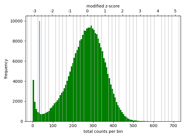
The correction diagnostic tool yielded a similar mad threshold within the range \([-3,-2]\). Even so, I followed the HicExplorer recommendation to set the lower threshold to at least -2 and the upper threshold to 5 in the pre-normalization filter. I argue that with a high number of valid contacts, it is safer to err on the side of caution and maybe filter out bad data.


The five samples were pooled with hicSumMatrices, and the non-standard contigs (unplaced scaffolds) were filtered out, and the different resolutions were created (hicMergeMatrixBins). HiCExplorer also comes with a normalization function prior to correcting the matrix, which should be applied if different samples should have comparable bin counts. It has no effect when having only one matrix. Nevertheless, the pooled matrix was normalized and then corrected compared in Figure 7. It is now obvious why we have to correct the matrix. The uncorrected (Figure 7 (a)) has no signal apart from the diagonal. Even though some bins have been filtered out, the expected plaid pattern of a contact matrix is visible along the diagonal after the correction (Figure 7 (b)), leaving evidence for chromatin structure, especially in the first 50 million bases of the chromosome. There is a wide region of empty values at the place of the centromere.
Eigenvectors
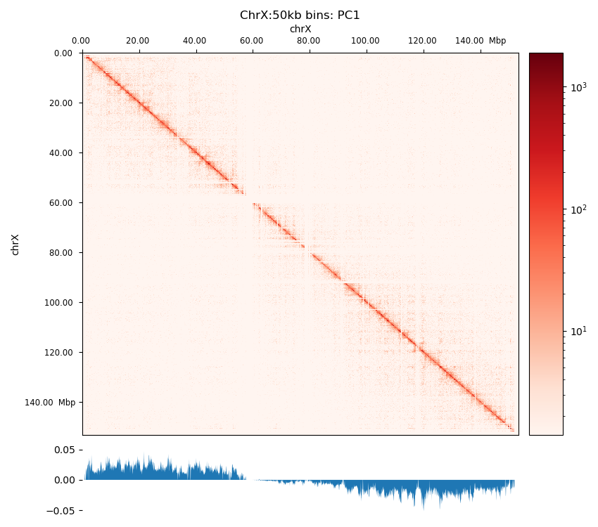
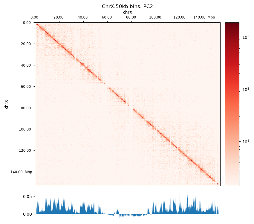
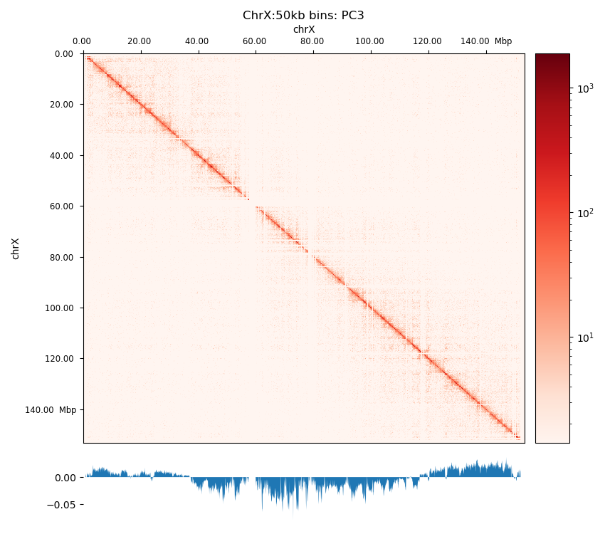
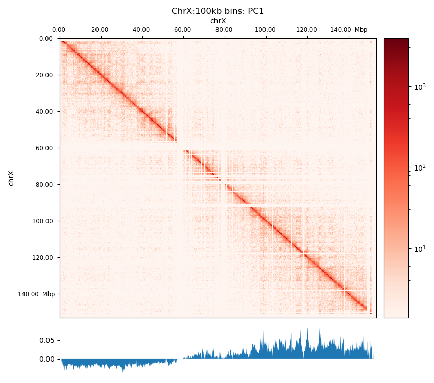
The PCA performed by hicPCA on the pooled samples at both 50kb and 100kb resolution yielded the first 3 principal components. For PC1 on both resolutions (Figure 8 (a), Figure 8 (d)) we observe only a single sign change which occurs at around 60 Mbp, the region of the centromere. It means the PCA has captured more variance between the chromosome arms than within them, making it uninformative about chromatin compartments. Upon visual inspection, it is clear that neither of the PC graphs capture the pattern of the interaction matrix by its change of sign. It seems the PCs capture variance from a bias that varies slowly and predictably along the chromosome. The first PC that is supposed to capture the compartments very suspiciously changes sign at the region of the centromere, a classic problem that could be solved by restricting the values from which the PC is calculated along the chromosome. Unimpressed, I rationalize that the option --extra-track to provide a gene track or histone coverage should not affect this result much. It should be provided as a phasing track to orient the eigenvector to positively correlate with gene density or histone marks, and could possibly muddle the compartments if not included. I followed HiCExplorer pipeline to plot and explore the matrices. At this point, I stoppped using HiCExplorer, as I assessed that a more flexible tool was needed.
Open2c ecosystem
Quality Control
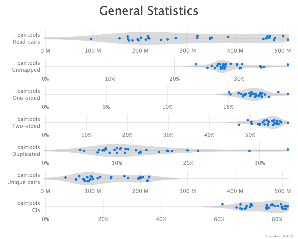
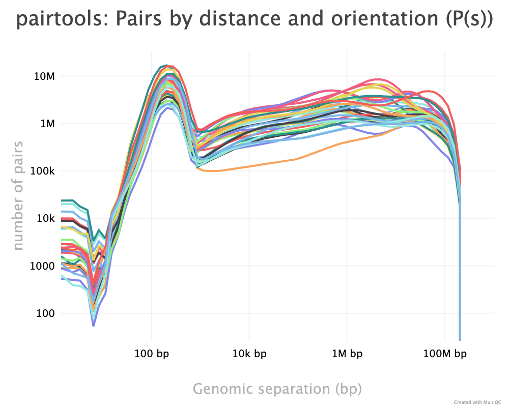
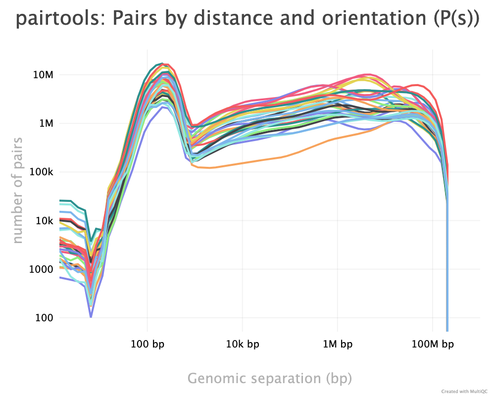
As described, the pairtools module in MultiQC was used to visualize results from pairtools stats for the two parsing runs, see Figure 9. The peak at around 250 bp is a techical artefact and should not be parsed into valid contacts.
--walks-policy mask
Comparing the multiQC report for each of the cell sources show similar distributions of unmapped (both sides unmapped), one-sided (one side mapped), two-sided (both sides mapped), and duplicated (w.r.t. total mapped) reads. The percentage of cis pairs w.r.t. mapped pairs is around 70% for all samples (Figure 9 (a)). The valid pairs also show similar distributions of pair types divided into 10 categories. The \(P(s)\) curve looks similar for all samples as well, peaking around 250 bp separation (Figure 9 (c)). The QC does not show any information about mapping quality of the reads. Note that the \(P(s)\) curve arise from pre-filtered pairs, meaning it provides information about the Hi-C library.
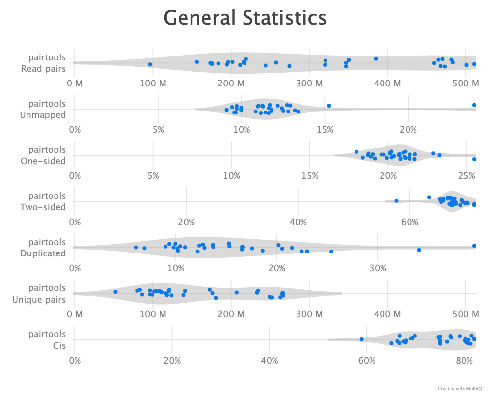
--walks-policy 5unique
Parsing alignments with the recommended walks-policy aproximately halves the percentage of unmapped reads, and one- and two-sided reads as well duplicated reads are slightly increased. Overall number of unique pairs are increased with more than 20% increase. The percentage of cis pairs are only decreased by a percentage point at most (Figure 9 (b)). Changing the walks policy does not alter the \(P(s)\) curve, meaning the parameter does not bias the parsing w.r.t. genomic separation.
--walks-policy mask
--walks-policy 5unique
--walks-policy mask
--walks-policy 5unique
pairtools stats run on all samples from the two walks-policies. Left (a+c): mask; right (b+d): 5unique. Generated by MultiQC (Ewels et al. 2016). Note: X-axes are not shared in the ‘Genereal Statistics’ plot.
Correction
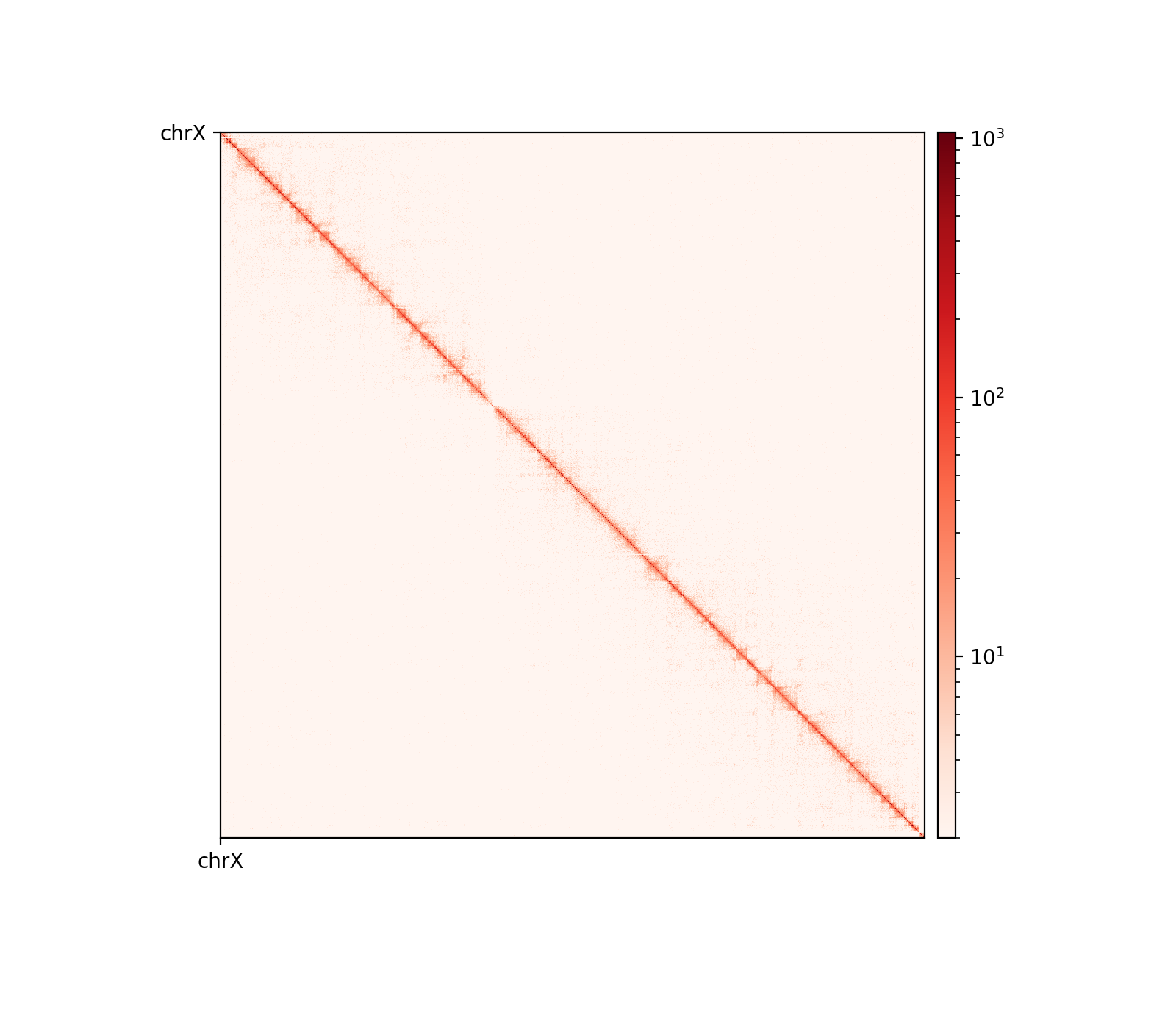
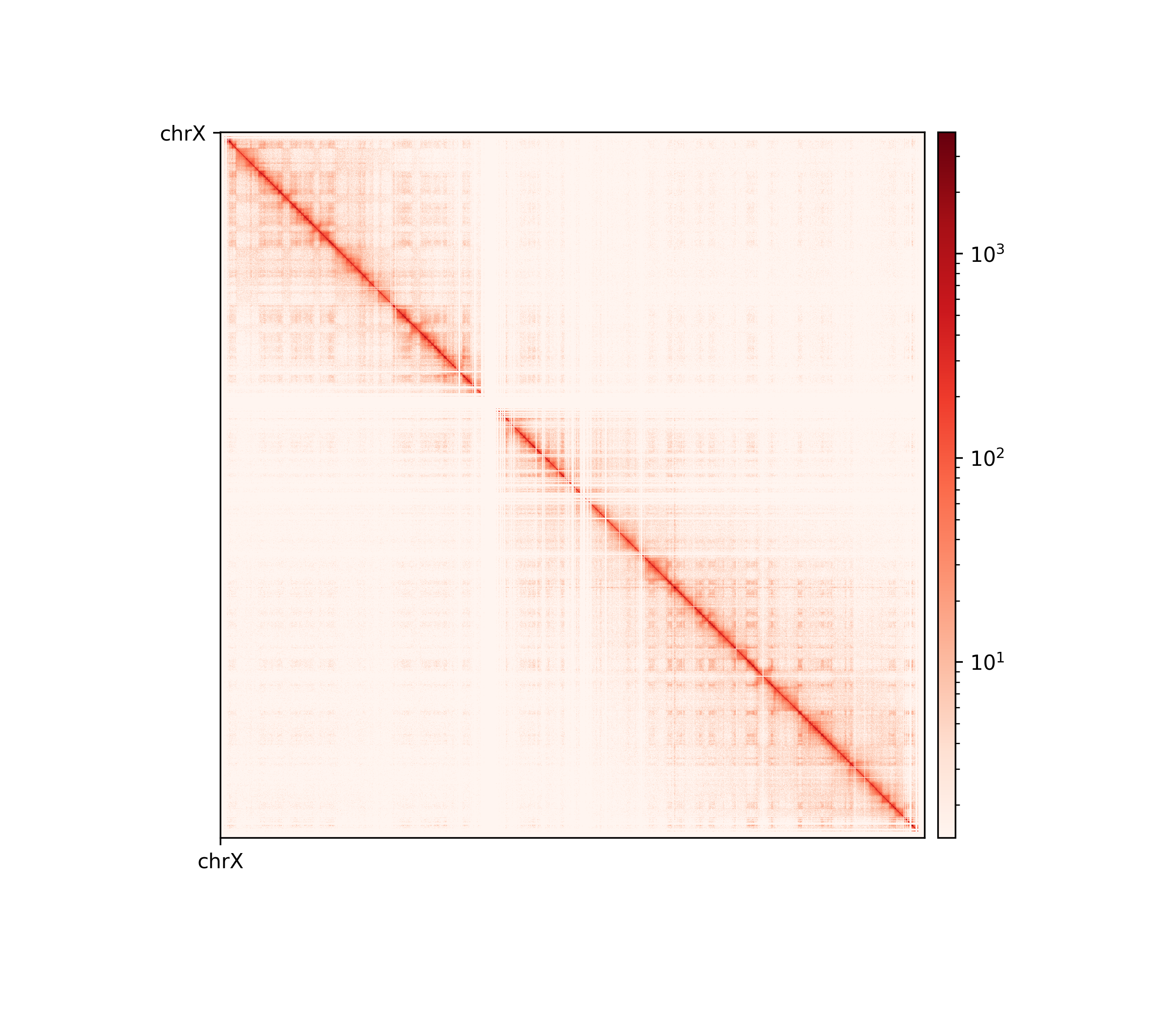
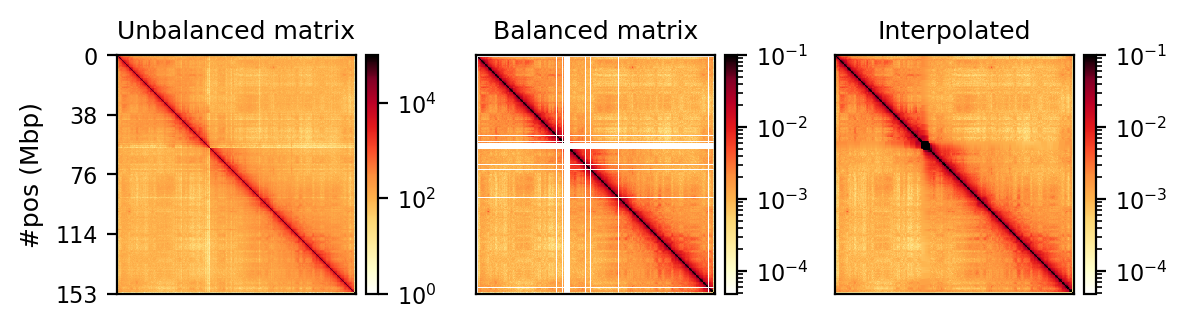
Matrix balancing did not show major improvement in the plaid pattern, as it already showed the expected pattern. It does, however, filter out bins that are deemed too low-count to be informative, for example peri-centromeric regions. The matrix was expected to be smoother after balancing (for chromosome-wide maps), as regions along a chromosome should only vary slowly in contact frequency with other regions as they are on a continouos molecule. Therefore, sharp contrasts represent a sudden drop in bin count (Figure 10 (a), raw) and should not be interpreted as devoid of interaction, but an indication that the data is not sufficient to interpret. It is then better to simply remove the bins instead of correcting, which will also amplify noise. Even with a high-quality Hi-C library we expect that all bins do not have the same coverage throughout(Lajoie, Dekker, and Kaplan 2015), as restriction enzymes do not bind equally to all regions of the genome, and therefore, some bins will be underrepresented as an artefact of binding/cutting efficieny of the restriction enzyme used.
We can try to mitigate the white lines of empty bins that now appear in the matrices. The coarsegrained and interpolated matrix is useful to make a good-looking interaction matrix, but is not that useful for analysis purposes. It might get easier to visually inspect the matrix, but it is not clear how well the interpolated matrix reflects the structure of the chromatin, and it is not transparent which regions are interpolated and which that are not. I find it purposeful for interpolation on high-resolution (zoomed-in) views (Figure 10 (b)) with small empty regions, but misleading for chromosome-wide maps, where typically the centromere and extremities of the chromosome have filtered-out bins. Interpolation is further discussed below.
The regions that are coarsegrained are small zero- or low-count bins which are averaged, effectively reducing the resolution of those regions until the count is sufficient. They get more frequent the longer genomic distance (the further we travel from the diagonal), and effectively enables us to get some intuition about the interactions. The coarsegrain, however, does not interpolate the NaNs created when filtering out whole bins in the balancing step (horisontal and vertical lines in Figure 10 (a) and Figure 10 (b); middle). This is done in a subsequent step by linearly interpolating the NaNs. Examining the interpolated matrix on full chrX (Figure 10 (a); right) gives the impression that the pericentromeric (at ~60 Mbp) region harbours a very strong compartment, but that is clearly an artefact of the interpolation on the very large empty region of the centromere, where the diagonal is somehow extended in a square. On the thinner lines, the interpolation seem to be more smooth, and barely noticable on the diagonal.

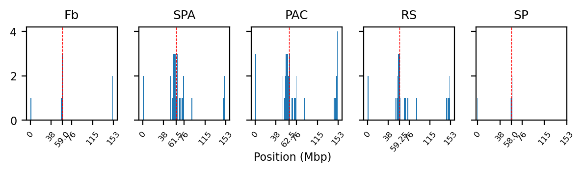
NaN histograms
As expected, most of the low quality bins are located on the edges of the chromosome arms, especially the region around the centromere (Warren et al. 2020), as they contain many repetitive sequences. The low-quality bins are filtered out by the balancing algorithm, those bins are NaN in the Hi-C matrix. The median position of the NaN values (Figure 11) ranges between \(58\) and \(63.5\), which is within the estimate of the centromeric region of rhemac10 (the UCSC browser has a continuously unannotated region at chrX:57,500,000-60,200,000). The fact that the medians lie within the centromeric region on all cell sources shows both that the majority of the bad bins are in the (peri)centromeric region and there are approximately equally many on each side.
Compartments (Eigenvectors)
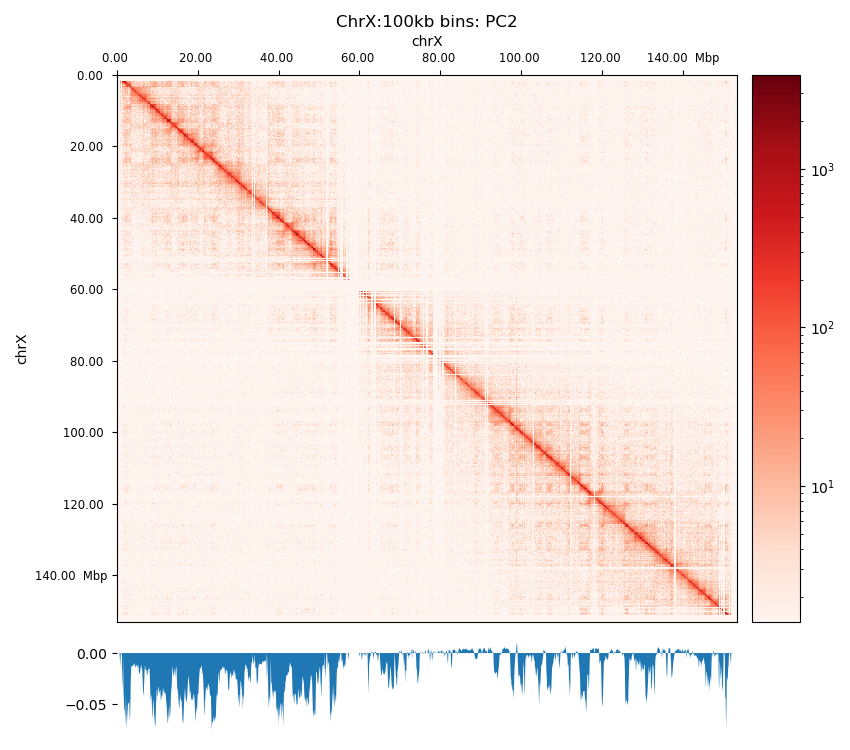
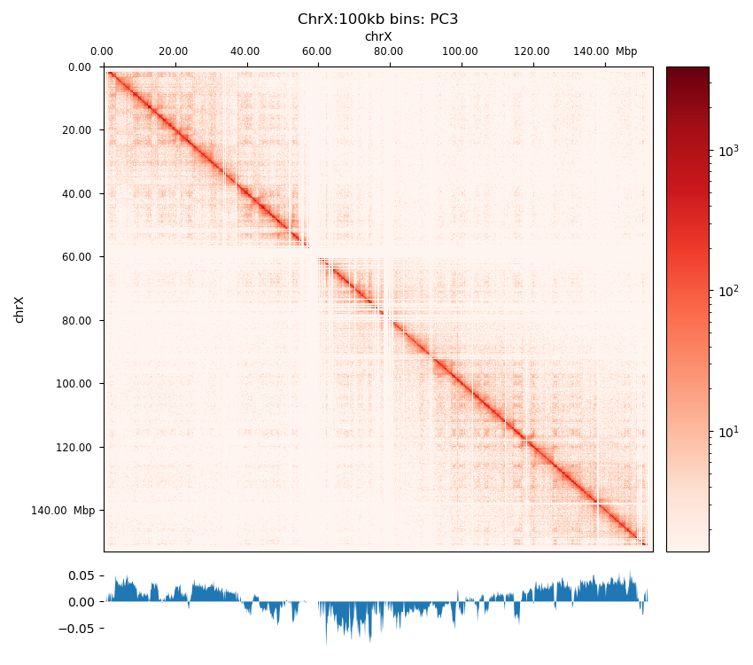
The three viewframes (Full, Arms, 10Mb) used for the calculation of the eigenvectors captured different variability in the data (Figure 12), and as expected, the inferred compartments (colored red on the E1 tracks) are more abundant and smaller with smaller viewframes. To determine how well each of the E1 tracks capture the pattern in the interaction matrix, we can overlay the matrix with the E1 sign-change and visually determine if the squares reflect the E1 sign change (Figure 12).
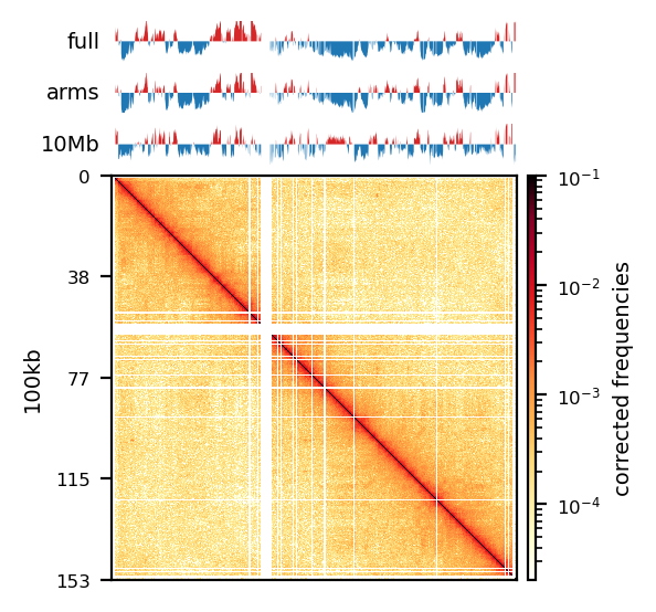
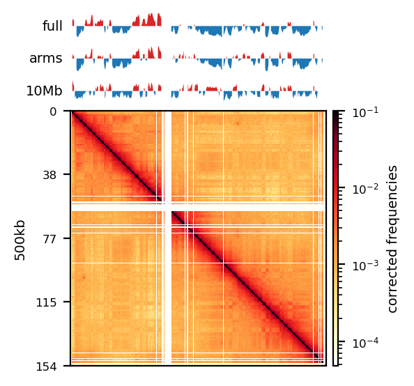
I decide that without more finescaled knowledge than the position of the centromeres, the arbitrary size of the 10 Mb windowed E1 can not fully be justified. That is, we could arbitrarily calculate any windowed E1 track. Also, Wang et al. (2019) concludes only for pachytene spermatocyte to show local interactions in the 10Mb viewframe (what they refer to as refined A/B-compartments), and all the other stages of spermatogenesis were consistent with the conventional A/B compartments. The reasonable thing to do is therefore to continue the analysis, focusing on the arms-restricted eigendecomposition. Nevertheless, we also keep refined compartments in the analysis.

5unique: chrX:start-end
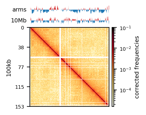
mask: chrX:start-end
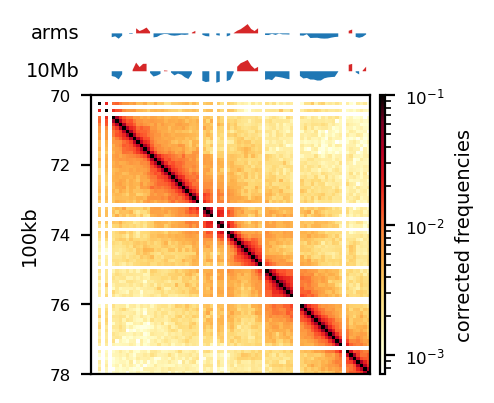
5unique: chrX:70Mb-78Mb
mask: chrX:70Mb-78Mb
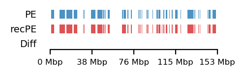
Additionally, as I created coolers with two different sets of parsing parameters we will compare the resulting matrices and their compartments (Figure 13). As expected, we observe more empty bins in the Hi-C matrix when comparing the initial run (mask) to the recommended parameters (5unique), but otherwise, the interaction pattern is indestinguishable. The effect on the E1 is more noticable, where the absolute magnitude of the E1 values is generally smaller. There is, however, a small region that changes sign (from A to B) on the 10Mb-windowed (‘refined’) E1 track (Figure 13;c+d). This region is surrounded by added empty bins, which could mean that too many low quality pairs in mask were introducing bias and swapped the sign of E1. It is supported by the fact that the sign change only occured in refined E1, and that the sign after filtering weak pairs (\(mapq < 30\)) is consistent with the arms view. It supports my previous postulate that it is better to use a viewframe with explicit molecular meaning than one of an arbitrary window size. That said, the mapq threshold should really be determined taking both coverage and resolution into account. For our purposes, and with the arms view, the mapping- and parsing parameters do not seem to be too sensitive.
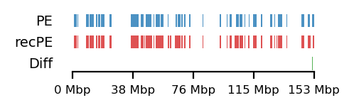
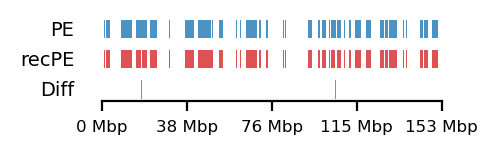
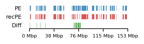
To emphasize the findings, the sets of A-compartments were compared between the two parsing runs, showing almost identical compartment calls. Additionally, the set difference was 8 bins between PE and recPE for round spermatid 100kb and 5 bins for fibroblast for arms viewframe (Figure 14; a+b, respectively). We observe a high number of differences around 76Mb for the refined compartments (10Mb) of round spermatid, which is consistent with the sign-flip of E1 values discussed earlier. Anything else would be surprising, as it is the same data, but visualized in a different way.
The observed difference between the sets can for our data be attributed to chance, but we cannot draw general conclusions about the parameters in general. I argue that the quality and size of the Hi-C library will influence sensitive to parsing parameters. In that case, the most flexible approach is still to follow the recommendations from cooler to report more pairs as valid contacts, and then create coolers with different mapq filters if issues are encountered.
Comparing Genomic Intervals
The comparison of genomic intervals was modified along the way, as we gained more knowledge and caught mistakes in the original implementation (especially of the proxomity test). Here, I only report the results of the final version of the software, but the modifications and implications hereof are discussed in Section 4.
Compartment Edges (transition zones)
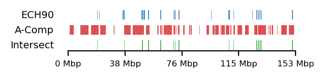
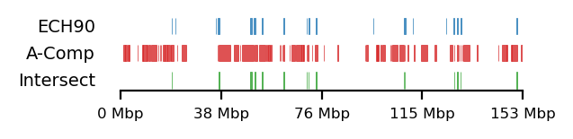
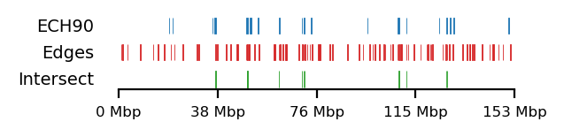
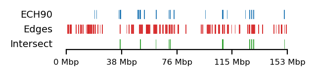
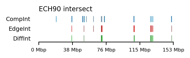
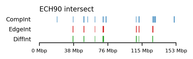
We compare how the ECH90 regions fit when queried on top of the A-compartments and equivalently for the edges, for fibroblasts and round spermatids at 100kb resolution. When queried against the edges instead, the the total set size is reduced to less than 50%. Interestingly, some of the intersections between A-compartments and ECH90 remain, and new ones appear as we move to the outside edge of the compartment (Figure 15). This indicates that most, but not all, of the intersection between ECH90 regions and the A-compartments are within 100kb of the compartment edge, and additional overlap is gained if we define a transition zone on the outside of the edge as well. To visualize this (outside) edge enrichment, we find the set difference of the ECH-intersection to compartments and edges, respectively (Figure 16), thus removing all the ‘inside’ edges. We observe that in almost all of the of the regions of \(ECH \cap Comp\) are accompanied by an edge also intersecting ECH (\(ECH \cap Edge\)), localized where the Diff track aligns (within 100kb) with both \(CompInt\) and \(EdgeInt\).
I apply both the proximity and Jaccard test to see how well the observations could be explained by chance. For completeness, the tests are performed for all cell types, but only use 100kb resolution and arms viewframe. We observe that both fibroblast and round spermatids have significant overlap (Jaccard p-values \(0.012\) and \(0.010\), respectively), meaning the edge zone have more intersection with the ECH regions than expected by chance. None of the samples passed the proximity test, meaning the non-overlapping segments were no more proximal than expected by chance. A significant proximity test (when performed on the edges) might provide information about the potential of expanding or moving the transition window. That is, if the non-overlapping regions are very proximal, a larger (or shifted) window to only capture the 200kb region outside of the edge might be favourable. With the very small amount of observed proximity (high p-values), we might consider shrinking the windows.
Testing against baboon regions under strong selection
The data for this analysis was provided by Kasper Munch in bed-like format, mapped to panu_3.0 (PapAnu4) assembly. The intervals define genomic regions in a hybrid/migrating population of baboon where strong negative selection acts against minor parent ancestry (Sørensen et al. 2023). The segments had to be lifted to rheMac10 coordinates to be able to correlate the two sets of intervals. The original UCSC-liftOver (Hinrichs 2006) is very strict and does not try to conserve segments in favor of accuracy e.g. inversions or small indels, which results in highly fragmented regions when lifted to another assembly, if the segments are not continouos on the new assembly. For our analysis, it is not the exact genomic position or order of sub-genic regions that are important, but rather, the start and end coordinates of each segment are quantified. To favor preservation of segments, we use segment_liftover (Gao, Huang, and Baudis 2018), resulting in much more similar segments to the original (Figure 17). As no chain file from panu_3.0 to Mmul_10 was available, we used panu_2.0 as intermediate.
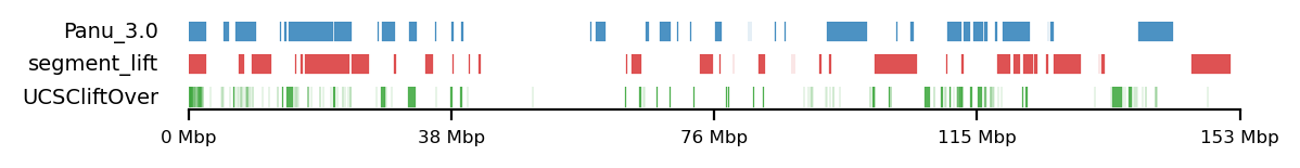
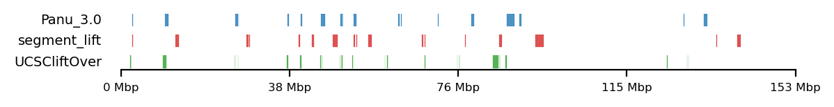
Initially, the compartment edges of round spermatid at 100kb resolution (RS100) were plotted against the lifted coordinates from the baboon hybrid population, where either all the sampled individuals have olive (P. anubis) ancestry or 95% of the sampled individuals have hamadryas (P. hamadryas ancestry. Their respective intersections were plotted underneath. We expect less intersection for hamadryas than for anubis as the total set size is much smaller. The compartment edges and Papio anubis-derived regions(Figure 18; b) seem to be highly enriched in the first 25 Mbp, and thus it has a high degree of intersection with the compartment edges. Interestingly, the ECH90 set is nearly empty in that region, which could be useful for determining the mechanism for selecting against the P.hamadryas ancestral allele in the hybrid baboon population. The P.hamadryas-derived regions seem intersect the compartment edges more centered on the chromosome (Figure 18; a). The proximity test initially ruled out that the non-intersecting parts of the respective regions were this proximal by chance. However, after updating the method to exclude whole segments that partially overlaps (instead of keeping their non-overlapping parts), there was no statistical significance. Additionally, the Jaccard test revealed that the intersection between the RS100 and both Hi-P.hama and Hi-P.anu can be explained by chance alone with no p-values below \(0.05\).
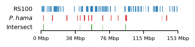
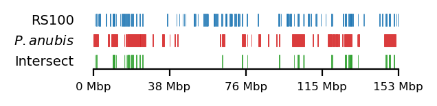
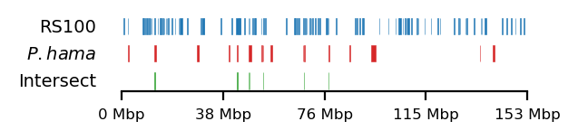
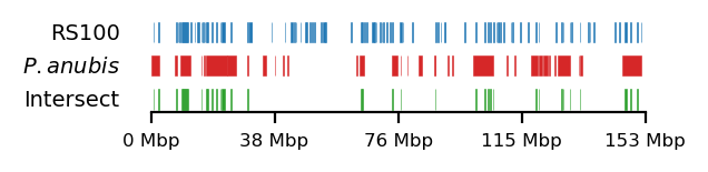
Testing limits
We then abandoned the idea of a 200kb transition zone between the compartments. It was introduced as a less stringent edge, allowing the intersection of the selected regions to be within a defined threshold. We hoped a weaker threshold could allow for more variance, but it turned out to be the opposite (Table 6). After defining the compartment limits (_edge_1bp), we perform tests on combinations of all five sources (fibroblast, spermatogonia, pachytene spermatocyte, round spermatid, sperm) and 2 viewframes (arms, 10Mb) and 5 queries. The queries were modified as such; the full ECH was used unmodified for the tests as it was already shown to overlap (Jaccard) fibroblast and round spermatid. hama and olive limits were used separately and as a concatenated set (hamaolive_edge_1pb), to increase the effect size, especially as the hama set is quite small compared to the rest of the sets. By their definition, olive and hama do not overlap, and can safely be concatenated (see Figure 1 for confirmation). Now, we observe significant p-values across all cell types.
Reassuringly, both fibroblast and round spermatid still have significant Jaccard p-values for the arms viewframe although the p-values have increased (to \(0.017\) and \(0.028\), respectively). Now, all tissues except sperm show significant overlap with ECH regions, especially spermatogonia and pachytene spermatocytes with p-values \(0.006\) and \(0.005\), respectively. Only fibroblast and spermatogonia significantly overlap the ECH region for both viewframes, indicating that their predicted compartments shift only minimally compared to the pachytene spermatocyte and round spermatid when narrowing the viewframe. Pachytene spermatocyte and round spermatid loose their significance when narrowing the viewframe, meaning their compartments are highly varied between the two views, and the same conclusion can be drawn about sperm, as it gains significance when the viewframe is narrowed. Interestingly, only sperm overlaps the baboon regions with olive ancestry, and no tissue overlaps with hamadryas ancestry. Conversely, when concatenating the olive and hamadryas sets to capture all selection in baboons, both spermatogonia, pachytene spermatocyte, and sperm are significantly proximal. Here, sperm, which is not proximal in the arms viewframe, has the lowest p-value (\(p=0.001\)).
Discussion
On Reproducibility
As an extensive reproducibility infrastructere became a major part of the project, I have to reflect upon the advantages it has, but also the consequences it inevitably brings along. First, reproducibility is the basis of scientific progression, and idealisticly it should come before the discovery itself. But let us not pretend that reproducibility is favored above hypothesis testing to be the driving forces of progression, and let us not pretend that it has a singular definition. There are many layers to reproducibility, and we do, of course, not need to host a website or to construct a single-command pipeline for reproducing the analysis to call a study reproducible. Additionally, the option only exist for analyses that are strictly computational. It is, however, very useful and can greatly improve downstream efficiency, and I find it important to at least explore the available options. If such a pipeline had existed, I would not have had to spend weeks to update the results of Wang et al. (2019) to reflect a more recent reference genome. With such a pipeline, it is now easy to extend the analysis to include more samples and other species. Additionally, if they had made the coordinates of the compartments available, I could probably have used them directly and start by comparing genomic intervals. Instead, this became a study more of Hi-C data analysis than comparing genomic intervals.
At the time of writing, the repository is almost there w.r.t. reproducibility, but still not quite. It only reproduces the final analysis done with bwa, pairtools, cooler, cooltools, and not the preliminary analyses comparing aligners and using HicExplorer. This is the intention, as most use-cases would not need the results of a preliminary methodological comparison. However, the workflows are saved under scripts/ and can be run from there, or they can be added to the main workflow.py as separate targets. A small amount of refactoring of the directory structure is required as well, because some files are fetched from a parent folder to the project directory. Additionally, the main workflow is intensive in I/O and could be heavily optimized by piping between commands instead of writing the outputs to file and reading the files from the next command. However, that would make it harder to debug, as no checkpoints are saved. It would not be as efficient use of resources, which are requested on target level, as the analysis would have to run as a single target. The different steps of the pipeline are either CPU-bound or RAM-bound, but rarely both, and it would take some experimenting to find the optimal compromise. Additionally, the computational steps between a raw .cool file and a balanced, multi-resolution .mcool are performed in a notebook, and the steps should be moved to the workflow. Then, a final target should be added to the workflow, executing all the notebooks (they are named in order), to generate the figures and tables that are used in this manuscript and on the main project pages.
There is a major downside when trying to conform to an idealistic framework—the generation of figures and tables. Throughout this project, I have adhered to the rule that none of the figures and tables should be created or even annotated manually. It is very time-consuming to create production-quality figures that needs no further enhancements before embedding into a manuscript, and even more so do create tables that are both compatible with HTML and PDF. Here, Quarto inherits the limitations of Pandoc (which it uses internally to convert Markdown to its output formats), and it does not work well with complex grouped tables generated in Python to translate into LaTeX (which again is an idealistic typesetting system). As Quarto is a relatively new framework (first release 2022-07-28 Quarto Team (2022)), there are contiously released updates to fix bugs. Therefore, one can spend hours on a workaround for a feature, which could be included in week’s release.
I believe it is an important exercise to force oneself to be cautious about design choices and explore the advantages and limitations of the tools we have available to communicate what we want to communicate.
On Methodology
HiCExplorer is a comprehensive software that consist of an extensive list of ready-made command line functions that calls Python source code. It is modular, except for the parsing of the aligned reads into a raw Hi-C matrix. The documentation provide an extensive list of options to pass to the commands. Nevertheless, they do not provide a Python API (or at least not any documentation thereof). The modules can be imported into a Python-session with standard import syntax, but there are no guiding help pages. Looking through source code revealed that one would have to do something like
to use the plotting function directly within a notebook. However, it would have to modified to stop saving the plots as files instead of sending them to the display, and it would still require reading from files. Clearly, it is not meant to be used directly within Python, as additionally, the CLI function simply is a wrapper for the main()-function of the module:
HiCExplorer is, however, also integrated into Galaxy (The Galaxy Community et al. 2024; Wolff et al. 2020, 2018), a web-based platform that has computationally demanding softwares executable through their servers. Here, one can make a drag-and-drop workflow with HicExplorer’s commands, get integrated visualizations, among other cool stuff. Although it was not suitable for this project, they should be given credit for such an extensive integration. Additionally, following a Galaxy-walkthrough would have given me a better intuition of the pipeline they recommend, and faster as well.
The Open2C Ecosystem consists of three major modules—pairtools, cooler, and cooltools. They all conform to the same standards; they are highly modular, and highly flexible and extensively documented. They have an interactive cooler-demo running on Jupyter notebooks on a server, which is easily adaptable to other data. They include both a command-line interface and a (well-documented) Python API, where a Cooler class efficiently handles the Hi-C matrix. They provide tutorials on all 6 of their intended use cases—Visualization, Contacts vs Distance, Compartments and Saddleplots, Insulation and Boundaries, Dots and Focal Enrichment, and Pileups and Average Features—of which we only use visualization and compartments. The software is fully compatible with Pandas and Matplotlib packages, making the analysis highly flexible.
The drawback with having a very flexible tool is that the conventions are unclear. The latest methodological review is from 2015 (Lajoie, Dekker, and Kaplan 2015), and many things have progressed since then—a previously mentioned example being the update to bwa so mapping reads seperately is no longer necessary. Additionally, a Springer Protocol about Hi-C Data analysis (Bicciato and Ferrari 2022) is more recently published, but I find that it more so establishes a range of possibilities than a practical guideline.
On Results
The differences in the results the two tools produced were crucial, as I could not reproduce the eigenvector compartments reported in Wang et al. (2019) with HiCExplorer, as HiCExplorer has no (apparent) way of restricting the viewframe of the eigendecomposition. It resulted in highly biased PC-tracks that only resembled 2 or 3 compartments (Figure 8). While it is a strong limitation to the tool (either documentation-wise, or capability-wise), the Hi-C matrices were constructed in only a few steps and passed their the provided quality control, even though the mapping parameters were only explored superficially. The only notable deviance in quality control was a high fraction of valid contacts, but this may be relieved by increasing the default \(mapq\) threshold from \(15\) to \(30\) as the noted convention in Lajoie, Dekker, and Kaplan (2015). The contact matrices generated from HiCExplorer improved when correcting, but still, the visible pattern closely delimited by low-count bins. This undesirable feature may be mitigated by passing a stricter filtering threshold to hicCorrectMatrix.
The eigenvectors resulting from Open2C line up very well with the ones from Wang et al. (2019). Here, some of the maps were lined up and overlayed manually in a sketching software, as no coordinates were available from the authors. In hindsight, it could have been informative to request the analyzed datat from the authors. The predicted compartments from cooler qualitatively aligned very well with the ones predicted by Wang et al. (2019) if their track was split in the region of the centromere. I confidently rationalize that the reason I have to split in the centromeric region is the newly, more accurate reference genome. As it rheMac10 has closed a high amount of gaps since last reference (most of which are expected around the centromere), we expect more sequences to align in that region, resulting in a longer genome as well. This could readily have been tested by lifting the newly calculated coordinates to rheMac2, but I decided it was not worth the effort for a slightly more accurate (yet still qualitative) validation. Additionally, I wanted to shift the focus from reproducing their results to re-running their analysis on rheMac10. With similar reasoning, only a small effort was put into performing their exact eigendecomposition of the Hi-C matrices before abandoning, as it was deemed unnecessary to force a protocol that was not meant for the tool I was using.
Comparing the two separate runs for parsing parameters revealed only minor differences in parsing statistics, the most notable being the fraction of unmapped pairs, which was expected—a higher amount for mask than for 5unique. The lower amount of unmapped reads also seem to trigger a higher amount of duplicates. As a result, the two runs end up with the same distribution of cis pairs. Supporting the claim that the parsing parameters made no significant difference, the compartments called for each run were qualitatively compared (Figure 14), revealing only minor differences
The brief exploration of matrix plotting with Open2C shows how different measures that can be taken to improve visibility in some regions, but end up misrepresenting the data. Especially, for large genomic regions of missing values, the interpolation is very unreliable (Figure 10 (a), right), where it might be interpreted that very high-frequency interactions occur at the centromeric region. Additionally, as it does not add to the analysis, but only is for visualization, it looses transparency by hiding empty bins. The problem is not as evident in smaller regions (Figure 10 (b)), where mostly single empty bins are interpolated.
Narrowing the parameter space for testing
To mitigate the effects of multiple testing and reduce my own biases, I try to reason about the different parameters used to pick a subset of combinations to test for significant overlap (Jaccard test) or proximity. Comparing the corrected matrices with the calculated E1 values is initally a subjective task. I find that the predicted compartments are highly similar between arms and 10Mb views at both 100kb and 500kb resolutions, but with the full view of the chromosome, fewer compartments are determined. Bear in mind that none of the compartments can be said to be wrong, they all just capture the variance on different scales. Remembering that the size of the regions under selection were spanning 6 megabases at most informs the decision to discard the full genomic view, which is also supported by the litterature (Lajoie, Dekker, and Kaplan 2015), recommending partitioning the chromosome into its arms if the first eigenvector only captures the arms.
Similarly, the choice of resolution should be made cautiously. Here, the resolution of the matrix is the same resolution as the resolution of the eigenvector. Therefore, a resolution can be chosen to reflect the genomic scale that we want to investigate, and the minimum resolution required to test if the compartments overlap with regions under selection. Although some of these regions are exceptionally large, the shortest segment is just below 100 kb. Thus, the 100 kb resolution is deemed sufficient to capture compartments that are within the range of the regions under selection.
However, it is important to acknowledge the trade-offs involved in selecting a resolution. Higher resolutions (e.g., 50 kb or 10 kb) can provide finer detail and may help identify sub-compartmental structures or smaller features of chromatin organization. As Wang et al. (2019) used 40 kb matrices for TAD calling, resolution should not be an issue for 50 kb matrices in this context. Although this study did not experiment with higher resolutions than 100 kb, it is plausible that 50 kb resolution could better capture the structural variance. The sequencing depth and coverage of the library appear sufficient to support such analyses, further justifying the exploration of higher resolutions. On the other hand, lower resolutions (e.g., 500 kb or 1 Mb) are more robust for sparse datasets but may oversimplify chromatin structure and fail to resolve smaller regions under selection. The choice of 100 kb strikes a balance between these extremes, ensuring that biologically relevant features of both the compartments and the regions under selection can be detected while minimizing the risk of false positives due to noise.
It is thus apparent that further analysis at higher resolutions, such as 50 kb, could provide additional insights into the structural variance of the regions under selection. This study largely avoids performing in-depth quality control of the Hi-C library and the resulting interaction matrices, instead relying on qualitative evaluation. However, this approach is justified as I use the same resolution as Wang et al. (2019), whose work includes comprehensive quality control measures such as coverage profiles along the chromosomes, \(P(s)\) curves, and compartment segregation strength.
Correlating genomic regions
The extracted compartments and their 200 kb edge regions were qualitatively compared for overlap with the ECH region (Figure 15). For fibroblast (Fb) and round spermatid (RS), I observe promising overlap with ECH90. Additionally, visualization of the difference in overlaps (“DiffInt”) between (ECH, full compartments) and (ECH, edges) confirmed that the ‘outside’ edge captured additional overlap (see Figure 16). It would have been informative to compare the intersection of the same overlaps (“IntInt”) to determine whether the overlap occurs more frequently on the inside edge than the outside edge.
The Jaccard test confirmed significant ECH overlap with Fb and RS, with \(p=0.012\) and \(p=0.010\), respectively. In contrast, the proximity test showed no significant results, which is unsurprising given the design of the test. Specifically, when calculating the proximity index between a query and an annotation (query and annot, respectively), overlapping segments are masked from query before calculating the mean distance to the nearest non-overlapping segments. This means that substantial intersection, as confirmed by the Jaccard test, leads to many segments being removed in the proximity test. This design choice—–removing entire overlapping segments rather than just the overlapping bases–—creates a clearer separation between the two test statistics. Without this distinction, the proximity test could capture some of the variance inherent to the Jaccard statistic, making it harder to isolate proximal, non-overlapping segments.
The significant overlap between ECH regions, Fb, and RS at arms view is reproduced when testing at the compartment 1bp limits instead of the 200kb edges, although the significance is weakened a bit. The incresed p-value indicates that the full regions are important for for relationship. Surprisingly, the limits of both spermatogonia and pachytene spermatocyte are significantly overlapping the ECH regions, more so than both fibroblast and round spermatid, supporting the findings from Wang et al. (2019) that chromatin undergoes remodelling through spermatogenesis.
The visualization of the overlap between baboon regions and round spermatid showed notable amounts of intersection (Figure 18), but both significant overlap and proximity was rejected by the tests. Conversely, the tests performed on the 1bp limits of baboon regions against the 1bp limits of A/B compartments revealed a significant proximity between olive and spermatozoa. Additionally, significant proximity was observed between spermatogonia, pachytene spermatocyte by defining baboon regions under selection as a single set, olivehama, and here the significance was strengthened an order of magnitude for spermatozoa. This indicate that the effect size of the hama regions is too small for statistical inference, but also that the two sets of genomic intervals can be viewed as a single set, possibly indicating that similar forces have shaped the genomic landscape.
Notably, three out of five cell types both overlap the ECH regions and are proximal to the baboon limits—spermatogonia and spermatozoa in the 10Mb viewframe, and pachytene spermatocyte in the arms viewframe, indicating an indirect relationship through chromatin architecture. As neither proximity nor overlap is observed between the baboon regions and ECH, this observation could indicate that some structural features of the chromosome are aiding in reducing diversity. These findings propose an intricate relationship between chromatin architecture and evolutionary pressures. The intersection and proximity between regions under strong selection and chromatin compartments on the X chromosome of primates, along with their location on the X chromosome, suggest that structural genomic features influence patterns of diversity and selection. While these results are promising, further testing of the compartments is needed—both at higher resolutions and in other primates—to refine our understanding of these dynamics.
Notably, Skov et al. (2023) describe a compelling scenario where meiotic drive could explain the reduced diversity on ECH regions, and these structural features might also play a role in facilitating or constraining mechanisms like gene drive, which can significantly alter allele frequencies across generations by bypassing classical Mendelian inheritance. However, caution is warranted when inferring the role of gene drive, as it remains a contentious concept among biologists.
Gene Drive, Selfishness and its Effect on Selection
Gene drive occur when a particular collection of genes is propagated through a population by increasing the probability of transmitting genes to the offspring from random (Mendelian) inheritance, resulting in a biased gene transmission against its alternative (referred to as transmission advantage). Two categories of gene drivers exist (Bravo Núñez, Nuckolls, and Zanders 2018); class one drivers affect chromosome segregation in meiosis, and killer meiotic drivers will sabotage meiotic product that have not inherited the driving allele (Bravo Núñez, Nuckolls, and Zanders 2018). This happens regardless of the fitness effects of the developed organism, and is there often a factor offsetting classical selection. Even though the implications of such systems are potentially detrimental, they are notoriously difficult to detect. A circumstance contributing to the difficulty is that most genetic experiments are done in homozygotes. Bravo Núñez, Nuckolls, and Zanders (2018) state that the general choice of experimental system may have biased our understanding of sexual reproduction. A key point is; meiotic drivers can only be observed in heterozygotes, where a genetic driver has a competitor.
If an autosomal driver reaches fixation, it no longer has a target to act against, and consequently the driving phenotype will not be observed (Bravo Núñez, Nuckolls, and Zanders 2018). Over time, as there is neither selfish nor selective pressure to maintain the driving mechanism of a fixed driver, the mechanism will decay as it accumulates inactivating mutations. As a result, genetic drivers are said to be transient (Bravo Núñez, Nuckolls, and Zanders 2018) on an evolutionary timescale, unless it is linked to another positively selected allele (Jaenike 2001). Interestingly, gene drive is much more well-documented on sex chromosomes than for autosomes. Possibly because the sex chromosome meiotic drive inherently causes a skewed sex ratio, more notably raising a flag for further analysis. Or, because X and Y do not recombine, allowing for killer-supressor gene pairs to stay on separate chromosomes. The consequences of sex chromosome drive and skewed sex ratio can be widespread. A fully driving gene on X can to lead to the extinction of the population that fixes the allele (Jaenike 2001), as only one (fertile) offspring sex will be produced. Therefore, sex chromosome drivers usually exist in equilibrium with a supressor. When a population becomes female-biased, autosomal suppressors will be favored with a process termed Fisher’s sex ratio selection (Lindholm et al. 2016.), as the individuals that produce offspring of the minor-sex have higher fitness.
A driving element on X may target a region on Y, mitigating the risk of self-destruction and increasing its frequency at the same time. However, as it induces a skewed sex-ratio by limiting the number of functioning Y-bearing spermatozoa, the selection on Y to counter this effect is strong, engaging an evolutionary arms race between driving allele and its supressor, potentially explaining stable Y chromosome polymorphisms (Jaenike 2001). However, the Y chromosome only exist in the male population and a supressor on Y has only limited effect on the X chromosome on a population-scale compared to its autosomal cousins, which consequently often harbour supressors of X-drive, as they are passed down to more offspring than the Y chromosome. The fight between a driver and a supressor in their coevolution is linked to the chromosomal architecture, as they have been shown to be protected by low-recombining regions or chromosomal inversions, and to be mediating the evolution of karyotype (Lindholm et al. 2016). Thus, the structural features of a chromosome not only shield genetic drivers but influence the patterns of synteny, which, in turn, are shaped by both selection and genomic constraints.
The interplay between selfish genetic elements, such as gene drivers, and their suppression through coevolutionary processes emphasizes the importance of chromosomal architecture in shaping evolutionary dynamics. This evolutionary “arms race” between drivers and suppressors is not only driven by selection but also by the structural constraints of the chromosomes themselves. In particular, features such as low-recombining regions and chromosomal inversions offer a protective shield for these genetic elements, influencing both their persistence and their evolutionary trajectories. Given this, understanding the role of chromosomal organization in these dynamics can provide deeper insights into the mechanisms that govern selection on sex chromosomes and their broader genomic implications.
Conclusion and future work
In summary, I find that previously identified regions on X under strong selection in humans (referred to as ECHs) and in baboons (disproportionate P.hamadryas or P.anubis ancestry) strongly correlate with chromatin A/B-compartments in some stages of spermatogenesis in rhesus macaque (Macaca mulata) inferred by PCA from either a chromosome-arm (conventional) viewframe or a 10 Mb viewframe (local). The regions under selection are associated with regions of low diversity and low ILS on the X chromosome across all the great apes.
Briefly, an array of significant intersection and proximity is observed when comparing ECH regions baboon regions with the 1bp limit of A/B compartments. Most notably, spermatogonia, spermatozoa, and pachytene spermatocyte was both significantly proximal to baboon regions and intersecting ECH regions. This suggests relationship between strong selection and chromosomal architecture, and as the selection is specific on X, it could indicate sex-chromosome related mechanisms. A point against a meiosis-specific mechanisms is that fibroblast intersects the ECH regions, where fibroblast was used as a control-group for spermatogenesis in Wang et al. (2019).
I duly note that this is purely an explorative and correlational study, requiring further testing to conclude a relationship between chromosomal organization and selection, even if my analysis yields statistically significant results. To provide a more solid foundation for this inference, the next steps could include:
- Include compartment metadata in the correlation, such as weighing by insulation score, or filter out edges that have adjecent missing values
- Recall compartments using higher-resolution matrices, or call TADs
- Analyze Hi-C spermatogenesis data in other great ape species (e.g. baboons)
- Use a more distant relative as a control group (e.g. the mouse data from Wang et al. (2019))
Until then, let us remain cautious in our interpretations, recognizing the complexity of the systems at play and the need for further investigation to validate the potential links between chromosomal architecture and selective forces. In the meantime, let us appreciate the complexity of a multi-species correlation between selection and the 3D architecture of our chromosomes, a region of considerable interest with many aspects still to be understood and explored.
Bibliography
Abdennur, Nezar, and Leonid A Mirny. 2020. “Cooler: Scalable Storage for Hi-C Data and Other Genomically Labeled Arrays.” Edited by Jonathan Wren. Bioinformatics 36 (1): 311–16. https://doi.org/10.1093/bioinformatics/btz540.
Allaire, J. J., Charles Teague, Carlos Scheidegger, Yihui Xie, and Christophe Dervieux. 2024. “Quarto.” https://doi.org/10.5281/zenodo.5960048.
Anaconda Software Distribution. 2016. “Anaconda Software Distribution.” Computer software. https://anaconda.com.
Baker, Monya. 2016. “1,500 Scientists Lift the Lid on Reproducibility.” Nature 533 (7604): 452–54. https://doi.org/10.1038/533452a.
Bersaglieri, Todd, Pardis C. Sabeti, Nick Patterson, Trisha Vanderploeg, Steve F. Schaffner, Jared A. Drake, Matthew Rhodes, David E. Reich, and Joel N. Hirschhorn. 2004. “Genetic Signatures of Strong Recent Positive Selection at the Lactase Gene.” The American Journal of Human Genetics 74 (6): 1111–20. https://doi.org/10.1086/421051.
Bicciato, Silvio, and Francesco Ferrari, eds. 2022. Hi-C Data Analysis: Methods and Protocols. Vol. 2301. Methods in Molecular Biology. New York, NY: Springer US. https://doi.org/10.1007/978-1-0716-1390-0.
Bravo Núñez, María Angélica, Nicole L. Nuckolls, and Sarah E. Zanders. 2018. “Genetic Villains: Killer Meiotic Drivers.” Trends in Genetics 34 (6): 424–33. https://doi.org/10.1016/j.tig.2018.02.003.
Cowell, Finn. 2023. “100 Years of Haldane’s Rule.” Journal of Evolutionary Biology 36 (2): 337–46. https://doi.org/10.1111/jeb.14112.
DevTeam, SRA Toolkit. 2024. “SRA Toolkit.” Wiki. GitHub. https://github.com/ncbi/sra-tools/wiki/01.-Downloading-SRA-Toolkit. https://trace.ncbi.nlm.nih.gov/Traces/sra/sra.cgi?view=software.
Dixon, Jesse R., Inkyung Jung, Siddarth Selvaraj, Yin Shen, Jessica E. Antosiewicz-Bourget, Ah Young Lee, Zhen Ye, et al. 2015. “Chromatin Architecture Reorganization During Stem Cell Differentiation.” Nature 518 (7539): 331–36. https://doi.org/10.1038/nature14222.
Dutheil, Julien Y., Kasper Munch, Kiwoong Nam, Thomas Mailund, and Mikkel H. Schierup. 2015. “Strong Selective Sweeps on the X Chromosome in the Human-Chimpanzee Ancestor Explain Its Low Divergence.” Edited by Nick H. Barton. PLOS Genetics 11 (8): e1005451. https://doi.org/10.1371/journal.pgen.1005451.
Ewels, Philip, Måns Magnusson, Sverker Lundin, and Max Käller. 2016. “MultiQC: Summarize Analysis Results for Multiple Tools and Samples in a Single Report.” Bioinformatics 32 (19): 3047–48. https://doi.org/10.1093/bioinformatics/btw354.
Gao, Bo, Qingyao Huang, and Michael Baudis. 2018. “Segment_liftover : A Python Tool to Convert Segments Between Genome Assemblies.” F1000Research 7 (June): 319. https://doi.org/10.12688/f1000research.14148.2.
GenomeDK. 2023. “Gwf Workflow Manager.” https://github.com/gwforg/gwf.git.
GitHub, Inc. n.d. “GitHub.” https://github.com.
Haldane, J. B. S. 1922. “Sex Ratio and Unisexual Sterility in Hybrid Animals.” Journal of Genetics 12 (2): 101–9. https://doi.org/10.1007/BF02983075.
Hinrichs, A. S. 2006. “The UCSC Genome Browser Database: Update 2006.” Nucleic Acids Research 34 (90001): D590–98. https://doi.org/10.1093/nar/gkj144.
Imakaev, Maxim, Geoffrey Fudenberg, Rachel Patton McCord, Natalia Naumova, Anton Goloborodko, Bryan R Lajoie, Job Dekker, and Leonid A Mirny. 2012. “Iterative Correction of Hi-C Data Reveals Hallmarks of Chromosome Organization.” Nature Methods 9 (10): 999–1003. https://doi.org/10.1038/nmeth.2148.
IT, AU. n.d. “Your Guide to GAI Responsibly.” https://medarbejdere.au.dk/en/gai. Accessed January 9, 2025.
Jaenike, John. 2001. “Sex Chromosome Meiotic Drive.” Annual Review of Ecology and Systematics 32 (1): 25–49. https://doi.org/10.1146/annurev.ecolsys.32.081501.113958.
Kluyver, Thomas, Benjamin Ragan-Kelley, Fernando Pérez, Brian Granger, Matthias Bussonnier, Jonathan Frederic, Kyle Kelley, et al. 2016. “Jupyter Notebooks ? A Publishing Format for Reproducible Computational Workflows.” In Positioning and Power in Academic Publishing: Players, Agents and Agendas, edited by Fernando Loizides and Birgit Scmidt, 87–90. IOS Press. https://eprints.soton.ac.uk/403913/.
Lajoie, Bryan R., Job Dekker, and Noam Kaplan. 2015. “The Hitchhiker’s Guide to Hi-C Analysis: Practical Guidelines.” Methods (San Diego, Calif.) 72 (January): 65–75. https://doi.org/10.1016/j.ymeth.2014.10.031.
Li, Heng. 2013. “Aligning Sequence Reads, Clone Sequences and Assembly Contigs with BWA-MEM.” https://arxiv.org/abs/1303.3997.
Lieberman-Aiden, Erez, Nynke L. Van Berkum, Louise Williams, Maxim Imakaev, Tobias Ragoczy, Agnes Telling, Ido Amit, et al. 2009. “Comprehensive Mapping of Long-Range Interactions Reveals Folding Principles of the Human Genome.” Science 326 (5950): 289–93. https://doi.org/10.1126/science.1181369.
Lindholm, Anna K., Kelly A. Dyer, Renée C. Firman, Lila Fishman, Wolfgang Forstmeier, Luke Holman, Hanna Johannesson, et al. 2016. “The Ecology and Evolutionary Dynamics of Meiotic Drive.” Trends in Ecology & Evolution 31 (4): 315–26. https://doi.org/10.1016/j.tree.2016.02.001.
Mailund, Thomas, Kasper Munch, and Mikkel Heide Schierup. 2014. “Lineage Sorting in Apes.” Annual Review of Genetics 48 (1): 519–35. https://doi.org/10.1146/annurev-genet-120213-092532.
Misteli, Tom. 2020. “The Self-Organizing Genome: Principles of Genome Architecture and Function.” Cell 183 (1): 28–45. https://doi.org/10.1016/j.cell.2020.09.014.
Munch, Kasper. 2024. “Munch-Group.” https://munch-group.org/research.html.
“Open2C.” n.d. Resource. Open Chromosome Collective. https://open2c.github.io/. Accessed November 13, 2024.
Open2C, Nezar Abdennur, Sameer Abraham, Geoffrey Fudenberg, Ilya M. Flyamer, Aleksandra A. Galitsyna, Anton Goloborodko, Maxim Imakaev, Betul A. Oksuz, and Sergey V. Venev. 2022. “Cooltools: Enabling High-Resolution Hi-C Analysis in Python.” Bioinformatics. https://doi.org/10.1101/2022.10.31.514564.
Open2C, Nezar Abdennur, Geoffrey Fudenberg, Ilya M. Flyamer, Aleksandra A. Galitsyna, Anton Goloborodko, Maxim Imakaev, and Sergey V. Venev. 2024. “Pairtools: From Sequencing Data to Chromosome Contacts.” Edited by Ferhat Ay. PLOS Computational Biology 20 (5): e1012164. https://doi.org/10.1371/journal.pcbi.1012164.
Quarto Team, Posit. 2022. “Announcing Quarto, a New Scientific and Technical Publishing System.” Posit.
Ramírez, Fidel, Vivek Bhardwaj, Laura Arrigoni, Kin Chung Lam, Björn A. Grüning, José Villaveces, Bianca Habermann, Asifa Akhtar, and Thomas Manke. 2018. “High-Resolution TADs Reveal DNA Sequences Underlying Genome Organization in Flies.” Nature Communications 9 (1): 189. https://doi.org/10.1038/s41467-017-02525-w.
Sayers, Eric W, Evan E Bolton, J Rodney Brister, Kathi Canese, Jessica Chan, Donald C Comeau, Ryan Connor, et al. 2022. “Database Resources of the National Center for Biotechnology Information.” Nucleic Acids Research 50 (D1): D20–26. https://doi.org/10.1093/nar/gkab1112.
Skov, Laurits, Moisès Coll Macià, Elise Anne Lucotte, Maria Izabel Alves Cavassim, David Castellano, Mikkel Heide Schierup, and Kasper Munch. 2023. “Extraordinary Selection on the Human X Chromosome Associated with Archaic Admixture.” Cell Genomics 3 (3): 100274. https://doi.org/10.1016/j.xgen.2023.100274.
Sørensen, Erik F., R. Alan Harris, Liye Zhang, Muthuswamy Raveendran, Lukas F. K. Kuderna, Jerilyn A. Walker, Jessica M. Storer, et al. 2023. “Genome-Wide Coancestry Reveals Details of Ancient and Recent Male-Driven Reticulation in Baboons.” Science 380 (6648): eabn8153. https://doi.org/10.1126/science.abn8153.
Team, The Matplotlib Development. 2024. “Matplotlib: Visualization with Python.” Zenodo. https://doi.org/10.5281/ZENODO.10916799.
The Galaxy Community, Linelle Ann L Abueg, Enis Afgan, Olivier Allart, Ahmed H Awan, Wendi A Bacon, Dannon Baker, et al. 2024. “The Galaxy Platform for Accessible, Reproducible, and Collaborative Data Analyses: 2024 Update.” Nucleic Acids Research 52 (W1): W83–94. https://doi.org/10.1093/nar/gkae410.
Torvalds, Linus, and Junio C Hamano. 2005. Git: A Distributed Version Control System. https://git-scm.com.
Wang, Yao, Hanben Wang, Yu Zhang, Zhenhai Du, Wei Si, Suixing Fan, Dongdong Qin, et al. 2019. “Reprogramming of Meiotic Chromatin Architecture During Spermatogenesis.” Molecular Cell 73 (3): 547–561.e6. https://doi.org/10.1016/j.molcel.2018.11.019.
Warren, Wesley C., R. Alan Harris, Marina Haukness, Ian T. Fiddes, Shwetha C. Murali, Jason Fernandes, Philip C. Dishuck, et al. 2020. “Sequence Diversity Analyses of an Improved Rhesus Macaque Genome Enhance Its Biomedical Utility.” Science 370 (6523): eabc6617. https://doi.org/10.1126/science.abc6617.
Waskom, Michael. 2021. “Seaborn: Statistical Data Visualization.” Journal of Open Source Software 6 (60): 3021. https://doi.org/10.21105/joss.03021.
Wolff, Joachim, Vivek Bhardwaj, Stephan Nothjunge, Gautier Richard, Gina Renschler, Ralf Gilsbach, Thomas Manke, Rolf Backofen, Fidel Ramírez, and Björn A Grüning. 2018. “Galaxy HiCExplorer: A Web Server for Reproducible Hi-C Data Analysis, Quality Control and Visualization.” Nucleic Acids Research 46 (W1): W11–16. https://doi.org/10.1093/nar/gky504.
Wolff, Joachim, Leily Rabbani, Ralf Gilsbach, Gautier Richard, Thomas Manke, Rolf Backofen, and Björn A Grüning. 2020. “Galaxy HiCExplorer 3: A Web Server for Reproducible Hi-C, Capture Hi-C and Single-Cell Hi-C Data Analysis, Quality Control and Visualization.” Nucleic Acids Research 48 (W1): W177–84. https://doi.org/10.1093/nar/gkaa220.
Zuo, Wu, Guangming Chen, Zhimei Gao, Shuai Li, Yanyan Chen, Chenhui Huang, Juan Chen, Zhengjun Chen, Ming Lei, and Qian Bian. 2021. “Stage-Resolved Hi-C Analyses Reveal Meiotic Chromosome Organizational Features Influencing Homolog Alignment.” Nature Communications 12 (1): 5827. https://doi.org/10.1038/s41467-021-26033-0.
A Appendix
Data Availability
All code, text, and files used for this project are available on https://github.com/munch-group/hic-spermatogenesis with instructions on how to reproduce.
Aknowledgements
People
I would like to extend my sincere gratitude to my supervisor, Kasper Munch, for his guidance and support throughout this project. His sparring and scientific literacy have been invaluable in refining my ideas and shaping the direction of this work. I am especially thankful for Kasper’s enthusiasm, which has been a source of motivation during this process. His expertise and insights were instrumental in setting up the Quarto templates and providing support for the discussion. His constructive feedback on the manuscript has greatly improved its quality. I feel fortunate to have had the opportunity to learn from and work with such a knowledgeable and dedicated mentor.
I would also like to thank my brothers, Jakob and Andreas, for their help with proofreading of the manuscript.
Compute
All computations were performed on GenomeDK (GDK), an HPC cluster located on Aarhus Uninversity, and most of the processing of the data was handled by a gwf workflow (GenomeDK 2023), a workflow manager developed at GDK. Developing the manuscript and all associated writing, editing, and rendering the project was also performed on GDK so work seemlesly with the analysis. I would like to thank GDK and Aarhus University for providing computational resources and support that contributed to these research results. None of this would have been possible on my own laptop from 2013.
Use of Generative Artificial Intelligence
As per Aarhus University guidelines (IT n.d.), I hereby disclose my use of Generative Artificial Intelligence (GAI) tools during the preparation of this thesis. All usage was conducted critically and responsibly, ensuring that the final work remained my own and adhered to academic integrity standards. These tools supplemented my expertise and accelerated routine tasks, but all creative, analytical, and scientific contributions are my own.
Copilot
I used Copilot for code completion and debugging, as well as modifying existing code to reflect updated variables and experimental needs.
ChatGPT
ChatGPT provided syntax support for Bash, YAML, JSON, Mermaid diagrams, and Pandoc Templates, to accelerate my learning of new programming languages. It hallucinates a lot about Quarto.
NotebookLM
NotebookLM supported the re-identification of references for a small amount of statements where placeholders ([ref]) were initially used before setting up BibTex references. Also to look up contradicting statements from other sources. NotebookLM only ‘knows’ the sources you provide it.
Footnotes
Bicciato and Ferrari (2022) mentions that this type of ligations had been used to model interaction between sister-chromatids post-replication in Drosophila.↩︎
And access to a high-performance computer with at least 12 TB storage and 32 CPU-cores, and a couple of days waiting time (else
gwf runwill fail as it asks for a lot of resources).↩︎