Detect selection in populations

library("ggplot2")
library("gridExtra")
library("ggpubr")
library("RColorBrewer")

RELATE

AFRICAN POPULATIONS

LWK <- read.table("/home/ari/ari-intern/people/ari/ariadna-intern/steps/LWK/relate/run_relate/1000g_ppl_phased_haplotypes_selection.sele", header = TRUE)
head(LWK)

A data.frame: 6 × 35

	pos	rs_id	X3571428.500000	X357142.937500	X257030.656250	X184981.281250	X133128.375000	X95810.585938	X68953.507812	X49624.847656	⋯	X257.030640	X184.981262	X133.128357	X95.810577	X68.953499	X49.624844	X35.714287	X0.000000	when_DAF_is_half	when_mutation_has_freq2
	<int>	<chr>	<int>	<int>	<int>	<int>	<int>	<int>	<dbl>	<dbl>	⋯	<dbl>	<dbl>	<dbl>	<dbl>	<dbl>	<dbl>	<dbl>	<int>	<dbl>	<dbl>
1	2781642	.	1	1	1	1	1	1	1	1	⋯	-0.1336880	-0.1734100	-0.2221450	-0.3321430	-0.3804730	-2.01040e-06	-0.000017053	0	-0.450077	-0.0978628
2	2781865	.	1	1	1	1	1	1	1	1	⋯	-2.4857200	-3.0492300	-1.8755900	-2.8888600	-2.4228300	-1.39308e+00	-1.576160000	0	-2.019680	-1.8051100
3	2781927	.	1	1	1	1	1	1	1	1	⋯	-0.0954429	-0.0623195	-0.0632732	-0.1635510	-0.4259450	-7.05956e-02	-0.034994400	0	-0.228440	-0.5814090
4	2782572	.	1	1	1	1	1	1	1	1	⋯	-0.1458270	-0.2778760	-0.3514220	-0.0907462	-0.0452048	-1.40217e-01	-0.176239000	0	-0.167312	-0.0570220
5	2783658	.	1	1	1	1	1	1	1	1	⋯	1.0000000	1.0000000	1.0000000	1.0000000	1.0000000	-4.91135e-01	-0.676691000	0	-1.409400	-0.4134500
6	2784657	.	1	1	1	1	1	1	1	1	⋯	-0.1243950	-0.1766240	-0.4322030	-0.4919260	-0.6999360	-7.43392e-01	-0.332010000	0	-0.212519	-1.0023100

LWK_plot <- plot(LWK$pos, -(LWK$when_mutation_has_freq2), pch = 19, col = "#8DA0CB", xlab = "Genomic Position", ylab = "log10(p-value)", main = "LWK",cex = 1.5, yaxp = c(0, 10, 5),cex.lab = 1.2)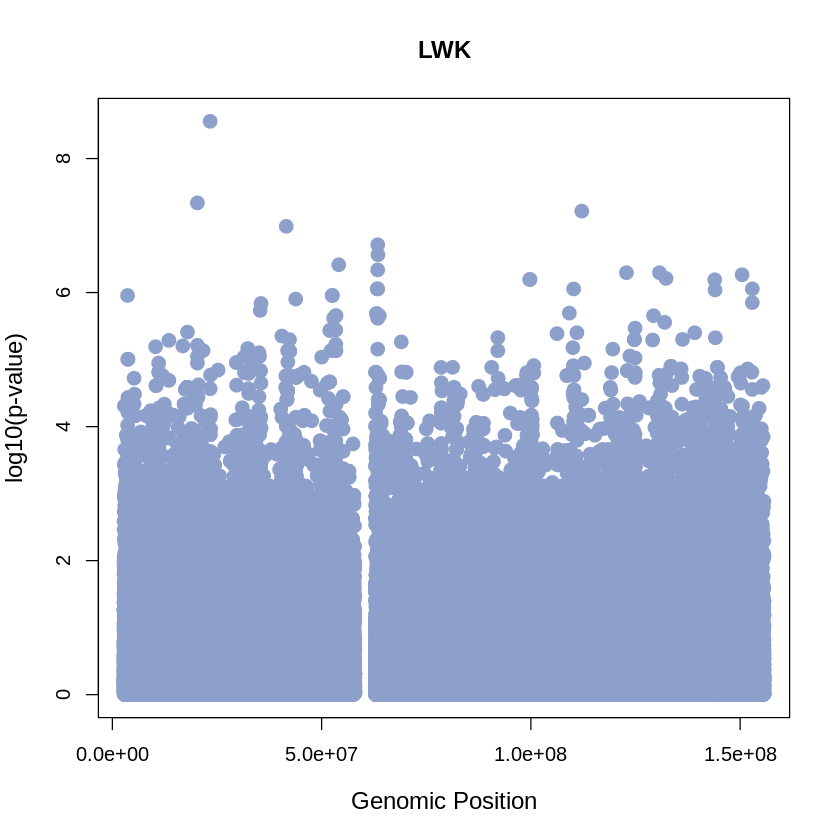

pdf("LWK_plot.pdf", width = 20, height = 5)
LWK_plot <- plot(LWK$pos, -(LWK$when_mutation_has_freq2), 
                 pch = 19, col = "#8DA0CB", 
                 xlab = "Genomic Position", 
                 ylab = "log10(p-value)", 
                 main = "LWK",
                 cex = 1.5, 
                 yaxp = c(0, 10, 5),
                 cex.lab = 1.3,
                 cex.main = 1.6,  # Adjust title size
                 cex.axis = 1.2)  # Adjust axis numbers size

dev.off()

png: 2

ESN <- read.table("/home/ari/ari-intern/people/ari/ariadna-intern/steps/ESN/relate/run_relate/1000g_ppl_phased_haplotypes_selection.sele", header = TRUE)
head(ESN)

A data.frame: 6 × 35

	pos	rs_id	X3571428.500000	X357142.937500	X257030.656250	X184981.281250	X133128.375000	X95810.585938	X68953.507812	X49624.847656	⋯	X257.030640	X184.981262	X133.128357	X95.810577	X68.953499	X49.624844	X35.714287	X0.000000	when_DAF_is_half	when_mutation_has_freq2
	<int>	<chr>	<int>	<int>	<int>	<int>	<int>	<int>	<dbl>	<dbl>	⋯	<dbl>	<dbl>	<dbl>	<dbl>	<dbl>	<dbl>	<dbl>	<int>	<dbl>	<dbl>
1	2781514	.	1	1	1	1	1	1	1	1	⋯	-0.241670	-0.163302	-0.211304	-0.385895	-0.654856	-0.342752	-0.492519	0	-0.418871	-0.757029
2	2781584	.	1	1	1	1	1	1	1	1	⋯	-0.327150	-0.196983	-0.174943	-0.153555	-0.248025	-0.261389	-0.445471	0	-0.293212	-0.658046
3	2781635	.	1	1	1	1	1	1	1	1	⋯	-0.486129	-0.319048	-0.511543	-0.744948	-0.701433	-0.315941	-0.226448	0	-0.849279	-0.203300
4	2781642	.	1	1	1	1	1	1	1	1	⋯	-0.355773	-0.505792	-0.598037	-0.100054	-0.162419	-0.290461	-0.382397	0	-0.320757	-0.190161
5	2781865	.	1	1	1	1	1	1	1	1	⋯	-0.584338	-0.299828	-0.218171	-0.373706	-0.187458	-0.249755	-0.502119	0	-0.312090	-0.580090
6	2781927	.	1	1	1	1	1	1	1	1	⋯	-0.600341	-0.785731	-0.495711	-0.520437	-0.477516	-1.343730	-1.212490	0	-0.488977	-0.879552

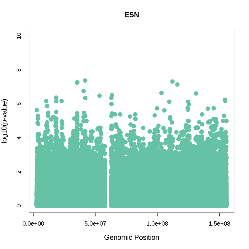
ESN_plot <- plot(ESN$pos, -(ESN$when_mutation_has_freq2), pch=19, col = "#66C2A5", xlab="Genomic Position", ylab="log10(p-value)", main ="ESN", cex = 1.5, ylim = c(0, 10), cex.lab = 1.2)
pdf("ESN_plot.pdf", width = 20, height = 5)
ESN_plot <- plot(ESN$pos, -(ESN$when_mutation_has_freq2), 
                 pch = 19, col = "#66C2A5", 
                 xlab = "Genomic Position", 
                 ylab = "log10(p-value)", 
                 main = "ESN",
                 cex = 1.5, 
                 yaxp = c(0, 10, 5),
                 cex.lab = 1.3,
                 cex.main = 1.6,  # Adjust title size
                 cex.axis = 1.2)  # Adjust axis numbers size

dev.off()

png: 2

GWD <- read.table("/home/ari/ari-intern/people/ari/ariadna-intern/steps/GWD/relate/run_relate/1000g_ppl_phased_haplotypes_selection.sele", header = TRUE)
head(GWD)

A data.frame: 6 × 35

	pos	rs_id	X3571428.500000	X357142.937500	X257030.656250	X184981.281250	X133128.375000	X95810.585938	X68953.507812	X49624.847656	⋯	X257.030640	X184.981262	X133.128357	X95.810577	X68.953499	X49.624844	X35.714287	X0.000000	when_DAF_is_half	when_mutation_has_freq2
	<int>	<chr>	<int>	<int>	<int>	<int>	<int>	<int>	<dbl>	<dbl>	⋯	<dbl>	<dbl>	<dbl>	<dbl>	<dbl>	<dbl>	<dbl>	<int>	<dbl>	<dbl>
1	2781514	.	1	1	1	1	1	1	1	1	⋯	-0.407876	-0.463329	-0.743589	-0.597593	-0.507644	-0.253240	-0.349971000	0	-0.614516	-0.656961
2	2781584	.	1	1	1	1	1	1	1	1	⋯	-0.179203	-0.154162	-0.180094	-0.205703	-0.124971	-0.231529	-0.204117000	0	-0.240526	-0.268348
3	2781635	.	1	1	1	1	1	1	1	1	⋯	-0.111829	-0.212617	-0.202914	-0.378425	-0.322488	-0.277704	-0.282409000	0	-0.190963	-0.782312
4	2781642	.	1	1	1	1	1	1	1	1	⋯	1.000000	-0.539265	-0.347216	-0.565445	-0.308591	-0.153304	-0.000101637	0	-0.686005	-0.379514
5	2781865	.	1	1	1	1	1	1	1	1	⋯	-0.519564	-0.462069	-0.316058	-0.352527	-0.137388	-0.134281	-0.264966000	0	-0.590395	-0.857276
6	2782386	.	1	1	1	1	1	1	1	1	⋯	-0.402728	-0.221762	-0.361282	-0.213686	-0.360681	-0.502329	-0.307497000	0	-0.555433	-0.201529

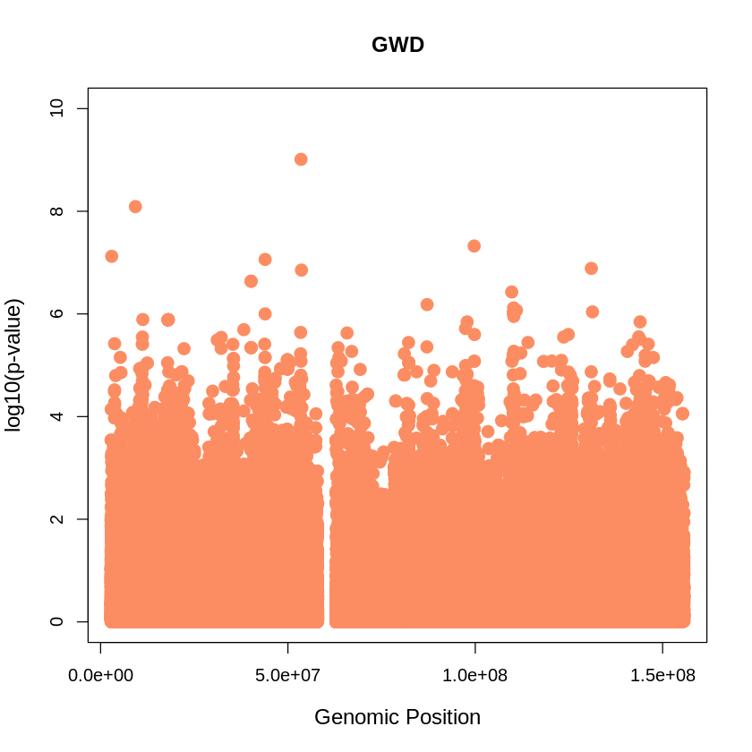
GWD_plot <- plot(GWD$pos, -(GWD$when_mutation_has_freq2), pch = 19, col = "#FC8D62", xlab = "Genomic Position", ylab = "log10(p-value)", main = "GWD", cex = 1.5, ylim = c(0, 10), cex.lab = 1.2)
pdf("GWD_plot.pdf", width = 20, height = 5)
GWD_plot <- plot(GWD$pos, -(GWD$when_mutation_has_freq2), 
                 pch = 19, col = "#FC8D62", 
                 xlab = "Genomic Position", 
                 ylab = "log10(p-value)", 
                 main = "GWD",
                 cex = 1.5, 
                 yaxp = c(0, 10, 5),
                 cex.lab = 1.3,
                 cex.main = 1.6,  # Adjust title size
                 cex.axis = 1.2)  # Adjust axis numbers size

dev.off()

png: 2

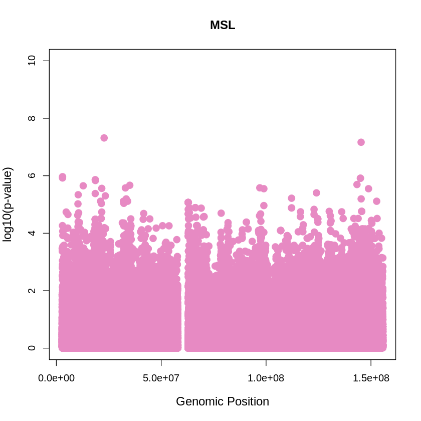
MSL <- read.table("/home/ari/ari-intern/people/ari/ariadna-intern/steps/MSL/relate/run_relate/1000g_ppl_phased_haplotypes_selection.sele", header = TRUE)
head(MSL)

A data.frame: 6 × 35

	pos	rs_id	X3571428.500000	X357142.937500	X257030.656250	X184981.281250	X133128.375000	X95810.585938	X68953.507812	X49624.847656	⋯	X257.030640	X184.981262	X133.128357	X95.810577	X68.953499	X49.624844	X35.714287	X0.000000	when_DAF_is_half	when_mutation_has_freq2
	<int>	<chr>	<int>	<int>	<int>	<int>	<int>	<int>	<dbl>	<dbl>	⋯	<dbl>	<dbl>	<dbl>	<dbl>	<dbl>	<dbl>	<dbl>	<int>	<dbl>	<dbl>
1	2781514	.	1	1	1	1	1	1	1	1	⋯	-0.00819344	-0.0230286	-0.0125319	-0.03071400	-0.0335299	-0.0137678	-0.0461147	0	-0.0346441	-0.1966720
2	2781584	.	1	1	1	1	1	1	1	1	⋯	-0.57859900	-0.6665050	-0.4813950	-0.19035200	-0.0996204	-0.3150730	-0.0203248	0	-0.6003820	-0.3105280
3	2781635	.	1	1	1	1	1	1	1	1	⋯	-0.48882200	-0.6708420	-0.4792100	-0.46056600	-0.7251980	-0.1401750	-0.2732000	0	-0.7939040	-1.4443700
4	2781865	.	1	1	1	1	1	1	1	1	⋯	-0.72332800	-0.4880510	-0.3577220	-0.49751700	-0.1608950	-0.2124540	-0.3456440	0	-0.7253440	-0.2675890
5	2781927	.	1	1	1	1	1	1	1	1	⋯	-0.40212600	-0.1816380	-0.2759440	-0.20043600	-0.1026650	-0.1161240	-0.1489970	0	-0.4218150	-0.4057530
6	2783658	.	1	1	1	1	1	1	1	1	⋯	-0.06384770	-0.0422283	-0.0282915	-0.00793583	-0.0163262	-0.0427755	0.0000000	0	-0.0417048	-0.0653668

MSL_plot <- plot(MSL$pos, -(MSL$when_mutation_has_freq2), pch = 19, col = "#E78AC3", xlab = "Genomic Position", ylab = "log10(p-value)", main = "MSL", cex = 1.5, ylim = c(0, 10), cex.lab = 1.2)
pdf("MSL_plot.pdf", width = 20, height = 5)
MSL_plot <- plot(MSL$pos, -(MSL$when_mutation_has_freq2), 
                 pch = 19, col = "#E78AC3", 
                 xlab = "Genomic Position", 
                 ylab = "log10(p-value)", 
                 main = "MSL",
                 cex = 1.5, 
                 yaxp = c(0, 10, 5),
                 cex.lab = 1.3,
                 cex.main = 1.6,  # Adjust title size
                 cex.axis = 1.2)  # Adjust axis numbers size

dev.off()

png: 2

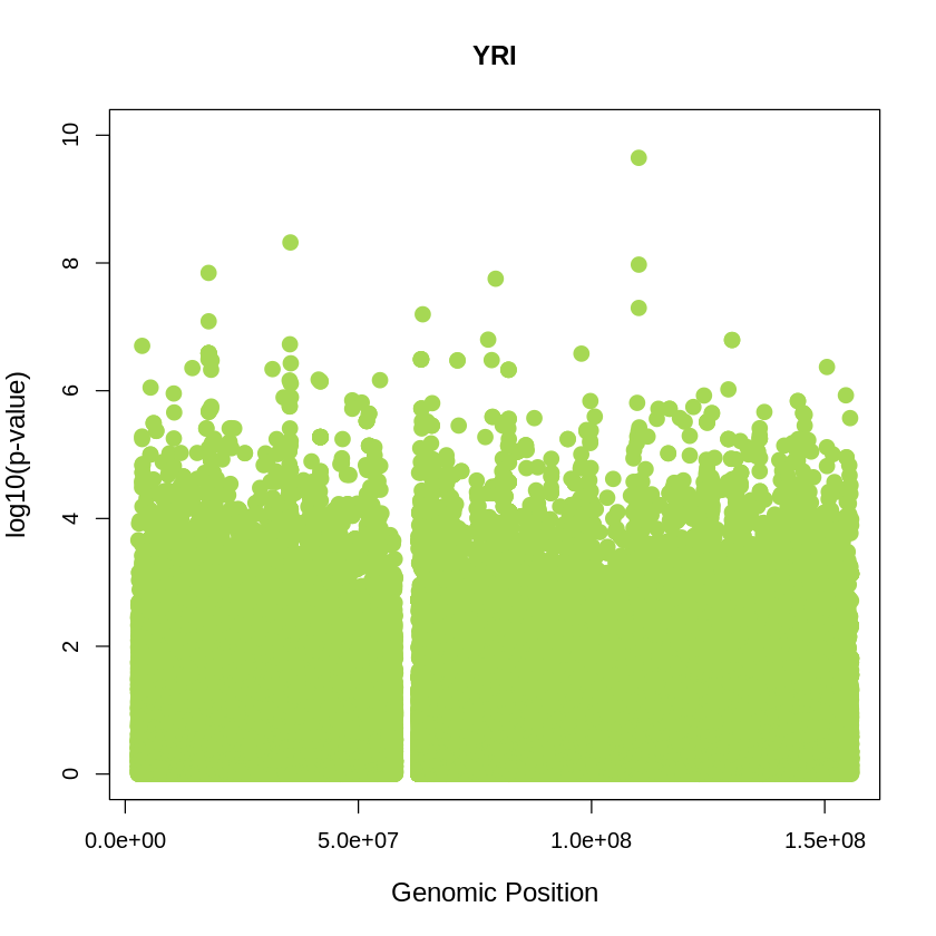
YRI <- read.table("/home/ari/ari-intern/people/ari/ariadna-intern/steps/YRI/relate/run_relate/1000g_ppl_phased_haplotypes_selection.sele", header = TRUE)
head(YRI)

A data.frame: 6 × 35

	pos	rs_id	X3571428.500000	X357142.937500	X257030.656250	X184981.281250	X133128.375000	X95810.585938	X68953.507812	X49624.847656	⋯	X257.030640	X184.981262	X133.128357	X95.810577	X68.953499	X49.624844	X35.714287	X0.000000	when_DAF_is_half	when_mutation_has_freq2
	<int>	<chr>	<int>	<int>	<int>	<int>	<int>	<dbl>	<dbl>	<dbl>	⋯	<dbl>	<dbl>	<dbl>	<dbl>	<dbl>	<dbl>	<dbl>	<int>	<dbl>	<dbl>
1	2781584	.	1	1	1	1	1	1	1	1	⋯	-1.202970	-0.649106	-1.2164900	-0.6031470	-0.860137	-1.338100	-1.0011900	0	-1.181280	-0.5485560
2	2781635	.	1	1	1	1	1	1	1	1	⋯	-0.174386	-0.318978	-0.0721344	-0.0799852	-0.184531	-0.190856	-0.3960370	0	-0.102744	-0.5156580
3	2781642	.	1	1	1	1	1	1	1	1	⋯	1.000000	1.000000	1.0000000	1.0000000	-0.621146	-0.869970	-1.2066100	0	-1.387990	-0.6117740
4	2781927	.	1	1	1	1	1	1	1	1	⋯	-0.668357	-0.674931	-0.6905980	-0.5737620	-0.274520	-0.216861	-0.3180610	0	-0.517044	-1.2772800
5	2782597	.	1	1	1	1	1	1	1	1	⋯	-0.262238	-0.398503	-0.5650450	-0.6882240	-0.131008	-0.191674	-0.0770765	0	-0.399880	-0.2131010
6	2783658	.	1	1	1	1	1	1	1	1	⋯	-0.514807	-0.961053	-0.9117400	-0.7238790	-1.248990	-1.566840	-1.3695800	0	-1.302540	-0.0112159

YRI_plot <- plot(YRI$pos, -(YRI$when_mutation_has_freq2), pch = 19, col = "#A6D854", xlab = "Genomic Position", ylab = "log10(p-value)", main = "YRI" , cex = 1.5, ylim = c(0, 10), cex.lab = 1.2)
pdf("YRI_plot.pdf", width = 20, height = 5)
YRI_plot <- plot(YRI$pos, -(YRI$when_mutation_has_freq2), 
                 pch = 19, col = "#A6D854", 
                 xlab = "Genomic Position", 
                 ylab = "log10(p-value)", 
                 main = "YRI",
                 cex = 1.5, 
                 yaxp = c(0, 10, 5),
                 cex.lab = 1.3,
                 cex.main = 1.6,  # Adjust title size
                 cex.axis = 1.2)  # Adjust axis numbers size

dev.off()

png: 2

# Combine data frames
LWK$Population <- "LWK"
ESN$Population <- "ESN"
GWD$Population <- "GWD"
MSL$Population <- "MSL"
YRI$Population <- "YRI"

combined_data <- rbind(LWK, ESN, GWD, MSL, YRI)

custom_theme <- theme_minimal() +
  theme(
    text = element_text(size = 14),  # Increase the text size for all text elements
    plot.title = element_text(size = 16, hjust = 0.5),  # Increase the title size
    axis.title = element_text(size = 15),  # Increase the axis label size
    axis.text = element_text(size = 12),  # Increase the axis text size
    legend.text = element_text(size = 14)  # Increase the legend text size
  )

# Create the plot
plot_combined <- ggplot(data = combined_data, aes(x = pos, y = -(when_mutation_has_freq2), color = Population)) +
  geom_point(pch = 19, size = 4) +
  labs(x = "Genomic Position", y = "log10(p-value)", title = "Africans") +
  theme_light() + custom_theme +
  geom_hline(yintercept = 6, color = "red") +
  scale_color_brewer(palette = "Set2") +
  theme(
    text = element_text(size = 15),
    plot.title = element_text(hjust = 0.5) # Center the title
  )

# Print the plot
print(plot_combined)

# Save the plot
ggsave("africans_threshold_REL_SQUARE.png", plot_combined, width = 7, height = 5)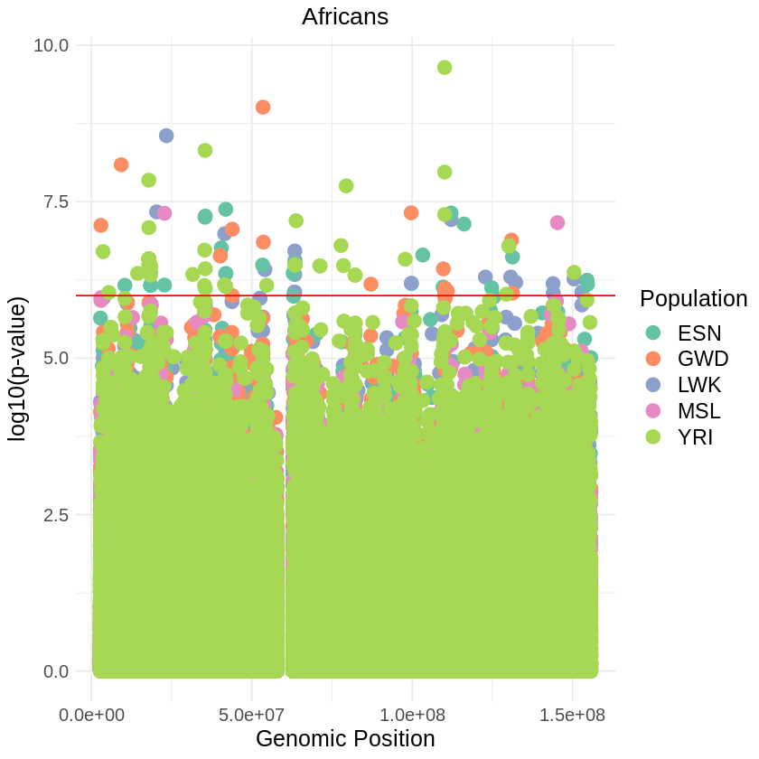

## SELECT JUST POSITION LOWER THAN THRESHOLD (log10 p-value < -6)

# Define file paths for the five .sele files
file_paths <- c(
  "/home/ari/ari-intern/people/ari/ariadna-intern/steps/LWK/relate/run_relate/1000g_ppl_phased_haplotypes_selection.sele",
  "/home/ari/ari-intern/people/ari/ariadna-intern/steps/ESN/relate/run_relate/1000g_ppl_phased_haplotypes_selection.sele",
  "/home/ari/ari-intern/people/ari/ariadna-intern/steps/GWD/relate/run_relate/1000g_ppl_phased_haplotypes_selection.sele",
  "/home/ari/ari-intern/people/ari/ariadna-intern/steps/MSL/relate/run_relate/1000g_ppl_phased_haplotypes_selection.sele",
  "/home/ari/ari-intern/people/ari/ariadna-intern/steps/YRI/relate/run_relate/1000g_ppl_phased_haplotypes_selection.sele"
)

# Read the files
LWK <- read.table(file_paths[1], header = TRUE)
ESN <- read.table(file_paths[2], header = TRUE)
GWD <- read.table(file_paths[3], header = TRUE)
MSL <- read.table(file_paths[4], header = TRUE)
YRI <- read.table(file_paths[5], header = TRUE)

# Function to subset data based on log10 p-value
subset_data <- function(data, population) {
  subset(data, when_mutation_has_freq2 < -6) %>%
    mutate(population = population)
}

# Define data frames and corresponding population names
file_pop <- list(
  list(data = LWK, population = "LWK"),
  list(data = ESN, population = "ESN"),
  list(data = GWD, population = "GWD"),
  list(data = MSL, population = "MSL"),
  list(data = YRI, population = "YRI")
)

# Subset and bind data from all files
africans_low_pvalue <- do.call(rbind, lapply(file_pop, function(fp) {
  subset_data(fp$data, fp$population)
}))

# Save the combined data to a single file
write.csv(africans_low_pvalue, "africans_low_pvalue.csv", row.names = FALSE)

filtered <- read.csv("/home/ari/ari-intern/people/ari/ariadna-intern/notebooks/africans_low_pvalue.csv")
head(filtered)
cat("Number of rows and columns:", paste(dim(filtered), collapse = "x"))

plot_threshold <- ggplot(filtered, aes(x = pos, y = -(when_mutation_has_freq2), color = population)) +
  geom_point(size = 4) +
  labs(x = "Genomic position", y = "log10 p-value", title = "AFRICAN") + 
  theme_minimal() + 
scale_color_brewer(palette = "Set2") + theme(text = element_text(size = 15),
        plot.title = element_text(hjust = 0.5))


print(plot_threshold)
ggsave("africans_low_pvalue_r.png", plot_threshold, width = 20, height = 8)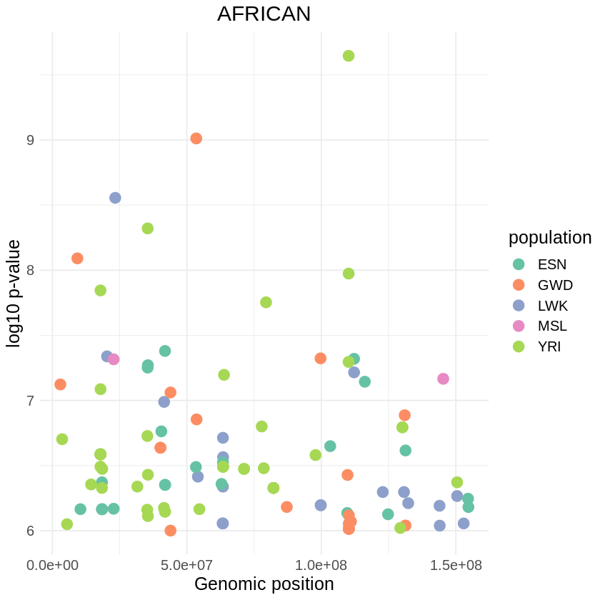

EUROPEAN POPULATIONS

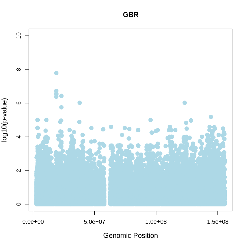
GBR <- read.table("/home/ari/ari-intern/people/ari/ariadna-intern/steps/GBR/relate/run_relate/1000g_ppl_phased_haplotypes_selection.sele", header = TRUE)
head(GBR)

A data.frame: 6 × 35

	pos	rs_id	X3571428.500000	X357142.937500	X257030.656250	X184981.281250	X133128.375000	X95810.585938	X68953.507812	X49624.847656	⋯	X257.030640	X184.981262	X133.128357	X95.810577	X68.953499	X49.624844	X35.714287	X0.000000	when_DAF_is_half	when_mutation_has_freq2
	<int>	<chr>	<int>	<int>	<int>	<int>	<int>	<int>	<dbl>	<dbl>	⋯	<dbl>	<dbl>	<dbl>	<dbl>	<dbl>	<dbl>	<dbl>	<int>	<dbl>	<dbl>
1	2781604	.	1	1	1	1	1	1	1	1	⋯	-0.04246550	-0.0410563	-0.0277191	0.00000000	0.0000000	0.0000000	0.000000	0	-0.0652181	-0.140835
2	2781635	.	1	1	1	1	1	1	1	1	⋯	-0.07381820	-0.0622531	-0.1658510	-0.20821400	-0.1090100	-0.2489250	0.000000	0	-0.2119610	-0.159586
3	2781927	.	1	1	1	1	1	1	1	1	⋯	-1.63264000	-1.4569200	-1.0390600	-1.39977000	-1.1803100	-0.5330060	-0.624974	0	-2.2223900	-1.710600
4	2781986	.	1	1	1	1	1	1	1	1	⋯	-1.63264000	-1.4569200	-1.0390600	-1.39977000	-1.1803100	-0.5330060	-0.624974	0	-2.2223900	-1.710600
5	2782116	.	1	1	1	1	1	1	1	1	⋯	-0.06384060	-0.0555249	-0.0357912	0.00000000	0.0000000	0.0000000	0.000000	0	-0.1008840	-0.372146
6	2782161	.	1	1	1	1	1	1	1	1	⋯	-0.00997385	-0.0102032	-0.0278379	-0.00742967	-0.0071796	-0.0841723	0.000000	0	-0.0321039	-0.141249

GBR_plot <- plot(GBR$pos, -(GBR$when_mutation_has_freq2), pch = 19, col = "lightblue", xlab = "Genomic Position", ylab = "log10(p-value)", main = "GBR" , cex = 1.5, ylim = c(0, 10), cex.lab = 1.2)
pdf("GBR_plot.pdf", width = 20, height = 5)
YRI_plot <- plot(GBR$pos, -(GBR$when_mutation_has_freq2), 
                 pch = 19, col = "lightblue", 
                 xlab = "Genomic Position", 
                 ylab = "log10(p-value)", 
                 main = "GBR",
                 cex = 1.5, 
                 yaxp = c(0, 10, 5),
                 cex.lab = 1.3,
                 cex.main = 1.6,  # Adjust title size
                 cex.axis = 1.2)  # Adjust axis numbers size

dev.off()

png: 2

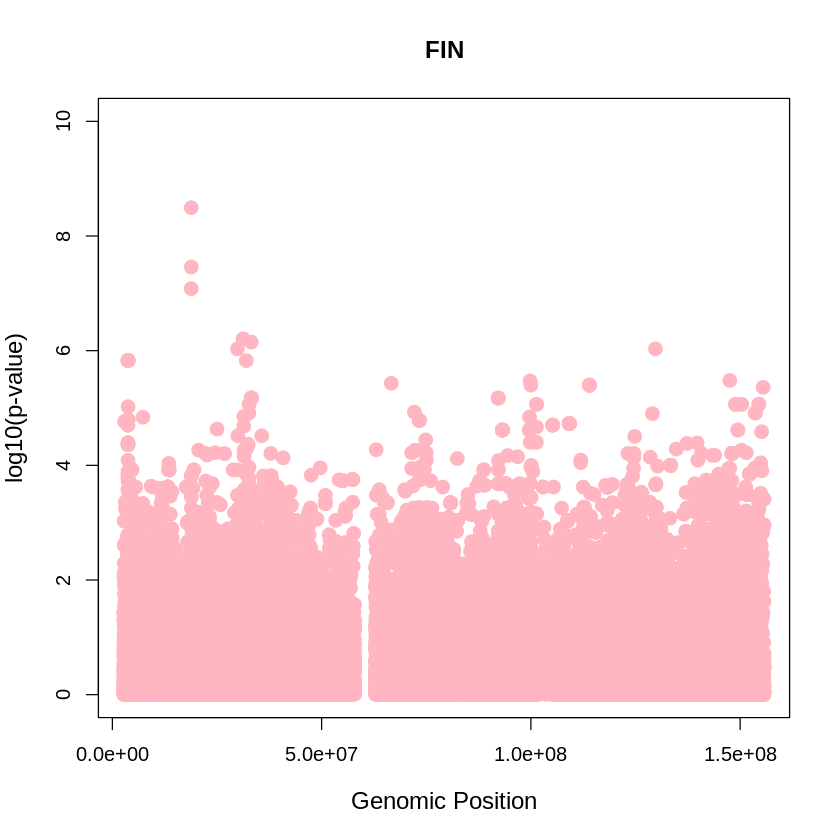
FIN <- read.table("/home/ari/ari-intern/people/ari/ariadna-intern/steps/FIN/relate/run_relate/1000g_ppl_phased_haplotypes_selection.sele", header = TRUE)
head(FIN)

A data.frame: 6 × 35

	pos	rs_id	X3571428.500000	X357142.937500	X257030.656250	X184981.281250	X133128.375000	X95810.585938	X68953.507812	X49624.847656	⋯	X257.030640	X184.981262	X133.128357	X95.810577	X68.953499	X49.624844	X35.714287	X0.000000	when_DAF_is_half	when_mutation_has_freq2
	<int>	<chr>	<int>	<int>	<int>	<int>	<int>	<int>	<dbl>	<dbl>	⋯	<dbl>	<dbl>	<dbl>	<dbl>	<dbl>	<dbl>	<dbl>	<int>	<dbl>	<dbl>
1	2781604	.	1	1	1	1	1	1	1	1	⋯	-0.00440755	-0.00534391	-0.0121758	-0.0395929	-0.12861100	-0.07316910	-4.72098e-05	0	-0.00567415	-0.0443709
2	2781635	.	1	1	1	1	1	1	1	1	⋯	-0.40902500	-0.62795400	-0.3375140	-0.4141800	-0.58893800	-0.68931200	-1.13840e+00	0	-0.57942200	-0.4660740
3	2781927	.	1	1	1	1	1	1	1	1	⋯	-0.65529300	-0.20453900	-0.2242660	-0.0580616	-0.00696292	-0.00380284	-3.23889e-03	0	-0.45251000	-1.3097700
4	2781986	.	1	1	1	1	1	1	1	1	⋯	-0.65529300	-0.20453900	-0.2242660	-0.0580616	-0.00696292	-0.00380284	-3.23889e-03	0	-0.45251000	-1.3097700
5	2782116	.	1	1	1	1	1	1	1	1	⋯	-0.00440755	-0.00534391	-0.0121758	-0.0395929	-0.12861100	-0.07316910	-4.72098e-05	0	-0.00567415	-0.0443709
6	2782161	.	1	1	1	1	1	1	1	1	⋯	-0.04182390	-0.09758080	-0.0624887	-0.1448340	-0.37536700	-0.37688400	-4.58744e-01	0	-0.03356820	-0.0363945

FIN_plot <- plot(FIN$pos, -(FIN$when_mutation_has_freq2), pch = 19, col = "lightpink", xlab = "Genomic Position", ylab = "log10(p-value)", main = "FIN" , cex = 1.5, ylim = c(0, 10), cex.lab = 1.2)
pdf("FIN_plot.pdf", width = 20, height = 5)
YRI_plot <- plot(FIN$pos, -(FIN$when_mutation_has_freq2), 
                 pch = 19, col = "lightpink", 
                 xlab = "Genomic Position", 
                 ylab = "log10(p-value)", 
                 main = "FIN",
                 cex = 1.5, 
                 yaxp = c(0, 10, 5),
                 cex.lab = 1.3,
                 cex.main = 1.6,  # Adjust title size
                 cex.axis = 1.2)  # Adjust axis numbers size

dev.off()

png: 2

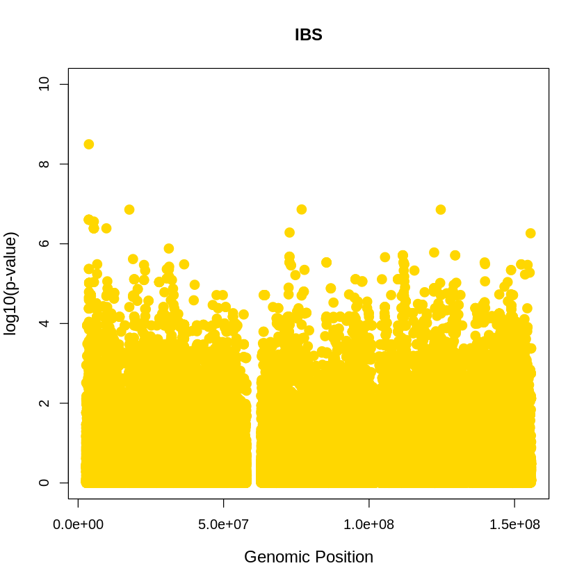
IBS <- read.table("/home/ari/ari-intern/people/ari/ariadna-intern/steps/IBS/relate/run_relate/1000g_ppl_phased_haplotypes_selection.sele", header = TRUE)
head(IBS)

A data.frame: 6 × 35

	pos	rs_id	X3571428.500000	X357142.937500	X257030.656250	X184981.281250	X133128.375000	X95810.585938	X68953.507812	X49624.847656	⋯	X257.030640	X184.981262	X133.128357	X95.810577	X68.953499	X49.624844	X35.714287	X0.000000	when_DAF_is_half	when_mutation_has_freq2
	<int>	<chr>	<int>	<int>	<int>	<int>	<int>	<int>	<dbl>	<dbl>	⋯	<dbl>	<dbl>	<dbl>	<dbl>	<dbl>	<dbl>	<dbl>	<int>	<dbl>	<dbl>
1	2781514	.	1	1	1	1	1	1	1	1	⋯	-0.5030530	-0.62381400	-0.6142110	-0.5986810	-0.2936090	-0.5673030	-0.5812090	0	-0.5659250	-0.430028
2	2781604	.	1	1	1	1	1	1	1	1	⋯	-0.1494370	-0.13499200	-0.0992126	-0.0863440	-0.0437142	-0.0229475	-0.0256627	0	-0.0950446	-0.487534
3	2781635	.	1	1	1	1	1	1	1	1	⋯	-0.6871990	-0.41871100	-0.4638830	-0.4103800	-0.7481900	-0.2844150	-0.4797510	0	-0.9172860	-0.408764
4	2781927	.	1	1	1	1	1	1	1	1	⋯	-0.0408422	-0.00879619	-0.0348159	-0.0113192	-0.0213689	-0.0237058	-0.1975070	0	-0.0570564	-1.165120
5	2781986	.	1	1	1	1	1	1	1	1	⋯	-0.0408422	-0.00879619	-0.0348159	-0.0113192	-0.0213689	-0.0237058	-0.1975070	0	-0.0570564	-1.165120
6	2782048	.	1	1	1	1	1	1	1	1	⋯	1.0000000	1.00000000	1.0000000	1.0000000	1.0000000	-0.9076720	-1.1323700	0	-1.5064100	-0.838322

IBS_plot <- plot(IBS$pos, -(IBS$when_mutation_has_freq2), pch = 19, col = "gold", xlab = "Genomic Position", ylab = "log10(p-value)", main = "IBS" , cex = 1.5, ylim = c(0, 10), cex.lab = 1.2)
pdf("IBS_plot.pdf", width = 20, height = 5)
IBS_plot <- plot(IBS$pos, -(IBS$when_mutation_has_freq2), 
                 pch = 19, col = "gold", 
                 xlab = "Genomic Position", 
                 ylab = "log10(p-value)", 
                 main = "IBS",
                 cex = 1.5, 
                 yaxp = c(0, 10, 5),
                 cex.lab = 1.3,
                 cex.main = 1.6,  # Adjust title size
                 cex.axis = 1.2)  # Adjust axis numbers size

dev.off()

png: 2

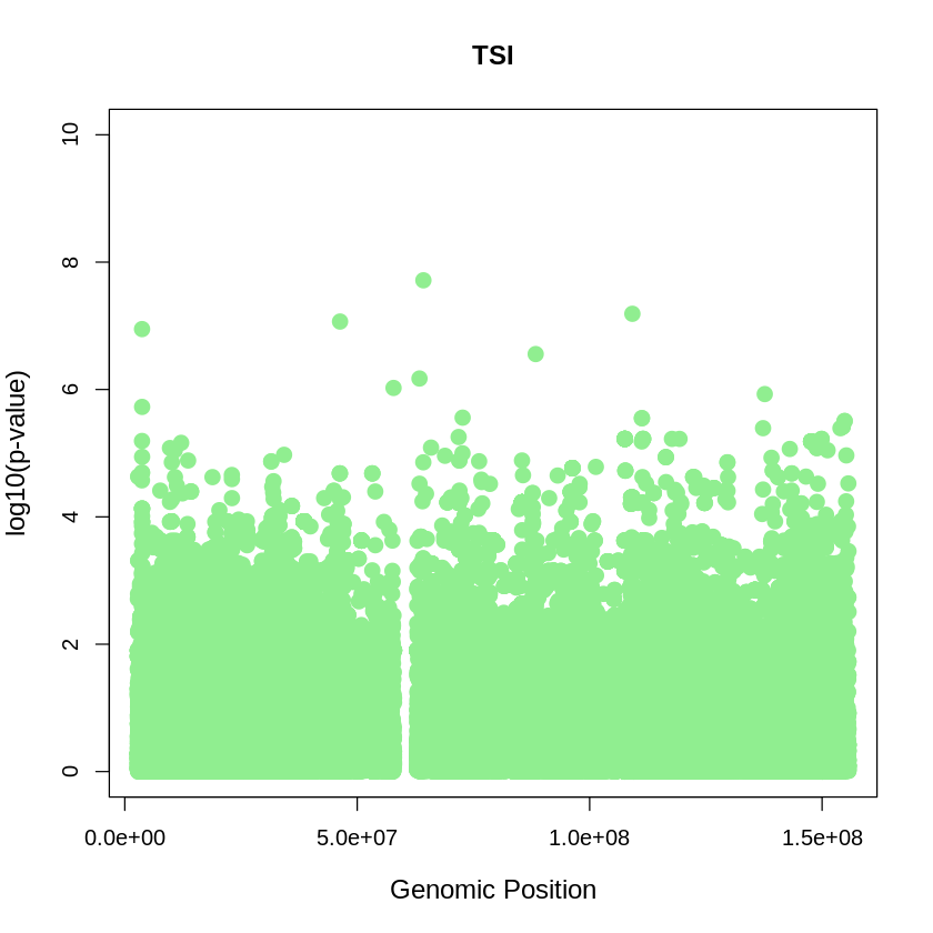
TSI <- read.table("/home/ari/ari-intern/people/ari/ariadna-intern/steps/TSI/relate/run_relate/1000g_ppl_phased_haplotypes_selection.sele", header = TRUE)
head(TSI)

A data.frame: 6 × 35

	pos	rs_id	X3571428.500000	X357142.937500	X257030.656250	X184981.281250	X133128.375000	X95810.585938	X68953.507812	X49624.847656	⋯	X257.030640	X184.981262	X133.128357	X95.810577	X68.953499	X49.624844	X35.714287	X0.000000	when_DAF_is_half	when_mutation_has_freq2
	<int>	<chr>	<int>	<int>	<int>	<int>	<int>	<int>	<dbl>	<dbl>	⋯	<dbl>	<dbl>	<dbl>	<dbl>	<dbl>	<dbl>	<dbl>	<int>	<dbl>	<dbl>
1	2781604	.	1	1	1	1	1	1	1	1	⋯	-0.2105130	-0.0994744	-0.00275779	-0.0264850	-0.1290760	-4.82756e-05	-2.05973e-05	0	-0.239337	-0.2886860
2	2781635	.	1	1	1	1	1	1	1	1	⋯	-0.0223887	-0.0254137	-0.05456920	-0.0224805	-0.0427598	-4.61010e-05	-2.00428e-05	0	-0.175876	-0.1633620
3	2781927	.	1	1	1	1	1	1	1	1	⋯	-1.7507600	-1.5958100	-2.17561000	-1.6023800	-0.9149070	-9.32056e-01	-1.16969e-01	0	-1.454490	-1.2938300
4	2781986	.	1	1	1	1	1	1	1	1	⋯	-1.7507600	-1.5958100	-2.17561000	-1.6023800	-0.9149070	-9.32056e-01	-1.16969e-01	0	-1.454490	-1.2938300
5	2782116	.	1	1	1	1	1	1	1	1	⋯	-0.1580850	-0.0765467	-0.00201294	-0.0222592	-0.1175840	-3.60871e-05	-1.89802e-05	0	-0.210797	-0.0313601
6	2782161	.	1	1	1	1	1	1	1	1	⋯	-0.3088920	-0.2460760	-0.54315200	-0.2379020	-0.5093210	-5.29402e-01	-1.07703e-01	0	-0.446141	-0.3001710

TSI_plot <- plot(TSI$pos, -(TSI$when_mutation_has_freq2), pch = 19, col = "lightgreen", xlab = "Genomic Position", ylab = "log10(p-value)", main = "TSI" , cex = 1.5, ylim = c(0, 10), cex.lab = 1.2)
pdf("TSI_plot.pdf", width = 20, height = 5)
TSI_plot <- plot(TSI$pos, -(TSI$when_mutation_has_freq2), 
                 pch = 19, col = "lightgreen", 
                 xlab = "Genomic Position", 
                 ylab = "log10(p-value)", 
                 main = "TSI",
                 cex = 1.5, 
                 yaxp = c(0, 10, 5),
                 cex.lab = 1.3,
                 cex.main = 1.6,  # Adjust title size
                 cex.axis = 1.2)  # Adjust axis numbers size

dev.off()

png: 2

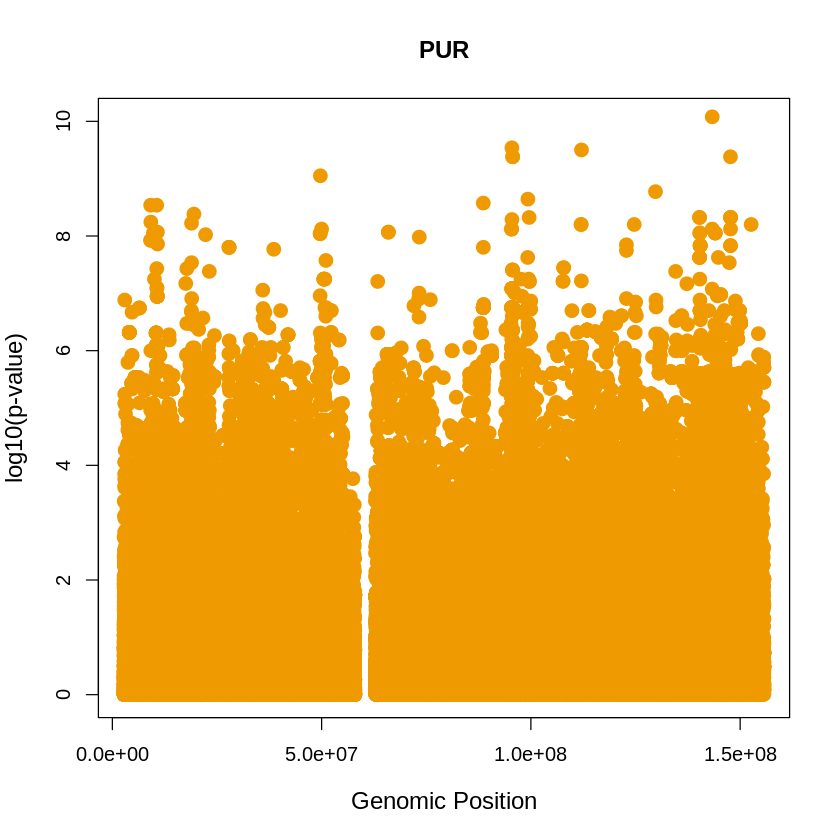
PUR <- read.table("/home/ari/ari-intern/people/ari/ariadna-intern/steps/PUR/relate/run_relate/1000g_ppl_phased_haplotypes_selection.sele", header = TRUE)
PUR_plot <- plot(PUR$pos, -(PUR$when_mutation_has_freq2), pch = 19, col = "orange2", xlab = "Genomic Position", ylab = "log10(p-value)", main = "PUR" , cex = 1.5, ylim = c(0, 10), cex.lab = 1.2)
pdf("PUR_plot.pdf", width = 20, height = 5)
PUR_plot <- plot(PUR$pos, -(PUR$when_mutation_has_freq2), 
                 pch = 19, col = "orange2", 
                 xlab = "Genomic Position", 
                 ylab = "log10(p-value)", 
                 main = "PUR",
                 cex = 1.5, 
                 yaxp = c(0, 10, 5),
                 cex.lab = 1.3,
                 cex.main = 1.6,  # Adjust title size
                 cex.axis = 1.2)  # Adjust axis numbers size

dev.off()

png: 2

# Combine data frames
GBR$Population <- "GBR"
FIN$Population <- "FIN"
IBS$Population <- "IBS"
TSI$Population <- "TSI"
PUR$Population <- "PUR"

combined_data <- rbind(GBR, FIN, IBS, TSI, PUR)


custom_theme <- theme_minimal() +
  theme(
    text = element_text(size = 14),  # Increase the text size for all text elements
    plot.title = element_text(size = 16, hjust = 0.5),  # Increase the title size
    axis.title = element_text(size = 15),  # Increase the axis label size
    axis.text = element_text(size = 12),  # Increase the axis text size
    legend.text = element_text(size = 14)  # Increase the legend text size
  )

plot_combined <- ggplot(data = combined_data, aes(x = pos, y = -(when_mutation_has_freq2), color = Population)) +
  geom_point(pch = 19, size = 4) +
  labs(x = "Genomic Position", y = "log10(p-value)", title = "Europeans + PUR") +
  theme_light() + custom_theme +
  geom_hline(yintercept = 6, color = "red") +
  scale_color_manual(values = c("GBR" = "lightblue", "FIN" = "lightpink", "IBS" = "gold", "TSI" = "lightgreen", "PUR" = "orange2")) + theme(text = element_text(size = 15)) 

print(plot_combined)

ggsave("europeans_threshold_REL_SQUARE.png", plot_combined, width = 7, height = 5)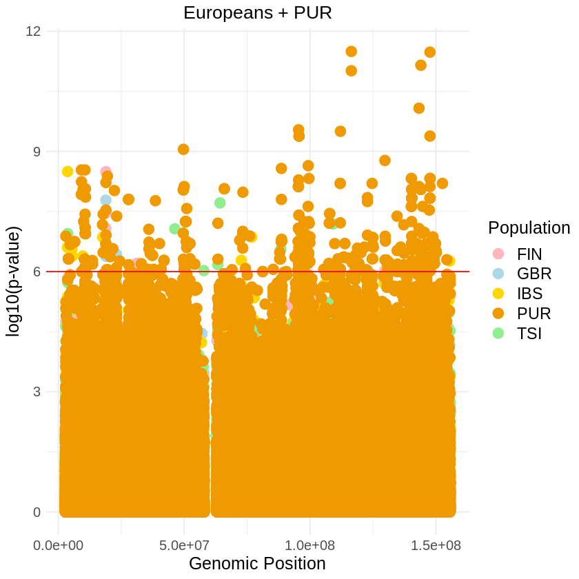

## SELECT JUST POSITION LOWER THAN THRESHOLD (log10 p-value < -6)

# Define file paths for the five .sele files
file_paths_euro <- c(
  "/home/ari/ari-intern/people/ari/ariadna-intern/steps/GBR/relate/run_relate/1000g_ppl_phased_haplotypes_selection.sele",
  "/home/ari/ari-intern/people/ari/ariadna-intern/steps/FIN/relate/run_relate/1000g_ppl_phased_haplotypes_selection.sele",
  "/home/ari/ari-intern/people/ari/ariadna-intern/steps/IBS/relate/run_relate/1000g_ppl_phased_haplotypes_selection.sele",
  "/home/ari/ari-intern/people/ari/ariadna-intern/steps/TSI/relate/run_relate/1000g_ppl_phased_haplotypes_selection.sele",
  "/home/ari/ari-intern/people/ari/ariadna-intern/steps/PUR/relate/run_relate/1000g_ppl_phased_haplotypes_selection.sele"
)

# Read the files
GBR <- read.table(file_paths_euro[1], header = TRUE)
FIN <- read.table(file_paths_euro[2], header = TRUE)
IBS <- read.table(file_paths_euro[3], header = TRUE)
TSI <- read.table(file_paths_euro[4], header = TRUE)
PUR <- read.table(file_paths_euro[5], header = TRUE)

# Function to subset data based on log10 p-value
subset_data <- function(data, population) {
  subset(data, when_mutation_has_freq2 < -6) %>%
    mutate(population = population)
}

# Define data frames and corresponding population names
file_pop <- list(
  list(data = GBR, population = "GBR"),
  list(data = FIN, population = "FIN"),
  list(data = IBS, population = "IBS"),
  list(data = TSI, population = "TSI"),
  list(data = PUR, population = "PUR")
)

# Subset and bind data from all files
europeans_low_pvalue <- do.call(rbind, lapply(file_pop, function(fp) {
  subset_data(fp$data, fp$population)
}))

# Save the combined data to a single file
write.csv(europeans_low_pvalue, "europeans_low_pvalue.csv", row.names = FALSE)

filtered_euro <- read.csv("/home/ari/ari-intern/people/ari/ariadna-intern/notebooks/europeans_low_pvalue.csv")
head(filtered_euro)
cat("Number of rows and columns:", paste(dim(filtered_euro), collapse = "x"))

A data.frame: 6 × 36

	pos	rs_id	X3571428.500000	X357142.937500	X257030.656250	X184981.281250	X133128.375000	X95810.585938	X68953.507812	X49624.847656	⋯	X184.981262	X133.128357	X95.810577	X68.953499	X49.624844	X35.714287	X0.000000	when_DAF_is_half	when_mutation_has_freq2	population
	<int>	<chr>	<int>	<int>	<int>	<int>	<int>	<int>	<int>	<int>	⋯	<dbl>	<dbl>	<dbl>	<dbl>	<dbl>	<dbl>	<int>	<dbl>	<dbl>	<chr>
1	18861677	.	1	1	1	1	1	1	1	1	⋯	-0.597739	-1.048370	-0.741127	-0.417716	-0.544644	-0.187459	0	-0.890654	-6.38066	GBR
2	18865240	.	1	1	1	1	1	1	1	1	⋯	-0.639418	-0.897673	-0.582284	-0.612257	-0.702097	-0.241534	0	-0.991791	-6.72386	GBR
3	18867826	.	1	1	1	1	1	1	1	1	⋯	-1.137600	-0.715037	-0.976634	-0.572180	-0.612715	-0.132271	0	-1.339690	-6.54745	GBR
4	18867954	.	1	1	1	1	1	1	1	1	⋯	-1.127090	-0.618784	-1.215980	-0.720713	-0.718903	-0.155134	0	-1.423040	-7.78284	GBR
5	18868013	.	1	1	1	1	1	1	1	1	⋯	-1.137600	-0.715037	-0.976634	-0.572180	-0.612715	-0.132271	0	-1.339690	-6.54745	GBR
6	18868321	.	1	1	1	1	1	1	1	1	⋯	-1.137600	-0.715037	-0.976634	-0.572180	-0.612715	-0.132271	0	-1.339690	-6.54745	GBR

Number of rows and columns: 456x36

plot_threshold <- ggplot(filtered_euro, aes(x = pos, y = -(when_mutation_has_freq2), color = population)) +
  geom_point(size = 4) +
  labs(x = "Genomic position", y = "log10 p-value", title = "European Populations") + 
  theme_minimal() + scale_color_manual(values = c("GBR" = "lightblue", "FIN" = "lightpink", "IBS" = "gold", "TSI" = "lightgreen", "PUR" = "orange2")) +
theme(text = element_text(size = 15),
        plot.title = element_text(hjust = 0.5))
print(plot_threshold)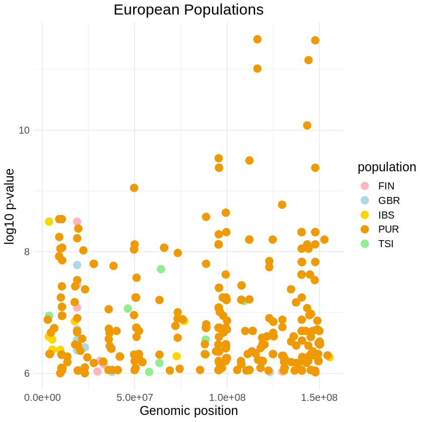

EAST ASIAN POPULATIONS

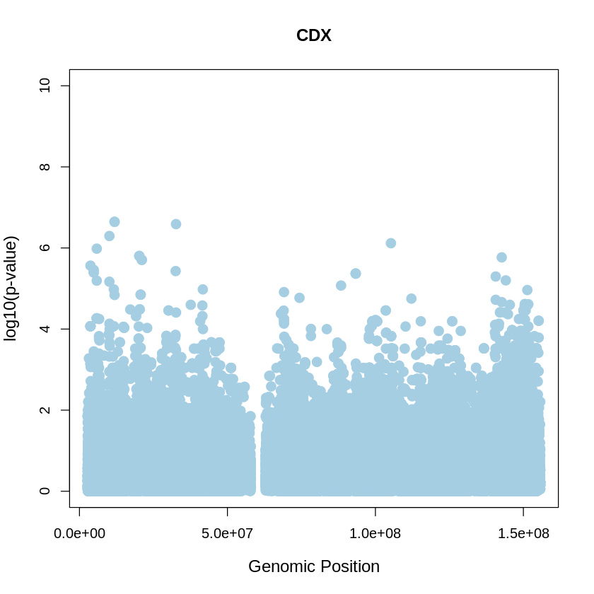
CDX <- read.table("/home/ari/ari-intern/people/ari/ariadna-intern/steps/CDX/relate/run_relate/1000g_ppl_phased_haplotypes_selection.sele", header = TRUE)
head(CDX)

A data.frame: 6 × 35

	pos	rs_id	X3571428.500000	X357142.937500	X257030.656250	X184981.281250	X133128.375000	X95810.585938	X68953.507812	X49624.847656	⋯	X257.030640	X184.981262	X133.128357	X95.810577	X68.953499	X49.624844	X35.714287	X0.000000	when_DAF_is_half	when_mutation_has_freq2
	<int>	<chr>	<int>	<int>	<int>	<int>	<int>	<int>	<dbl>	<dbl>	⋯	<dbl>	<dbl>	<dbl>	<dbl>	<dbl>	<dbl>	<dbl>	<int>	<dbl>	<dbl>
1	2781635	.	1	1	1	1	1	1	1	1	⋯	-1.0086400	-1.1085600	-1.1057000	-1.3585700	-0.943955	-1.1108200	-0.973984	0	-1.2454700	-0.4867200
2	2781927	.	1	1	1	1	1	1	1	1	⋯	-0.3131650	-0.2109630	-0.2253310	-0.0785041	-0.164815	-0.1097100	-0.108324	0	-0.3075960	-0.5534800
3	2781986	.	1	1	1	1	1	1	1	1	⋯	-0.3131650	-0.2109630	-0.2253310	-0.0785041	-0.164815	-0.1097100	-0.108324	0	-0.3075960	-0.5534800
4	2782161	.	1	1	1	1	1	1	1	1	⋯	-1.0339200	-1.0921500	-1.3285200	-1.5450600	-1.067340	-1.2125100	-1.057640	0	-1.2068300	-1.3679800
5	2782560	.	1	1	1	1	1	1	1	1	⋯	0.0000000	0.0000000	0.0000000	0.0000000	0.000000	0.0000000	0.000000	0	-0.0766008	-0.0269834
6	2782572	.	1	1	1	1	1	1	1	1	⋯	-0.0993169	-0.0502764	-0.0654512	-0.0539695	-0.238131	-0.0119095	-0.033889	0	-0.1106720	-1.6958700

CDX_plot <- plot(CDX$pos, -(CDX$when_mutation_has_freq2), pch = 19, col = "#A6CEE3", xlab = "Genomic Position", ylab = "log10(p-value)", main = "CDX" , cex = 1.5, ylim = c(0, 10), cex.lab = 1.2)
pdf("CDX_plot.pdf", width = 20, height = 5)
CDX_plot <- plot(CDX$pos, -(CDX$when_mutation_has_freq2), 
                 pch = 19, col = "#A6CEE3", 
                 xlab = "Genomic Position", 
                 ylab = "log10(p-value)", 
                 main = "CDX",
                 cex = 1.5, 
                 yaxp = c(0, 10, 5),
                 cex.lab = 1.3,
                 cex.main = 1.6,  # Adjust title size
                 cex.axis = 1.2)  # Adjust axis numbers size

dev.off()

png: 2

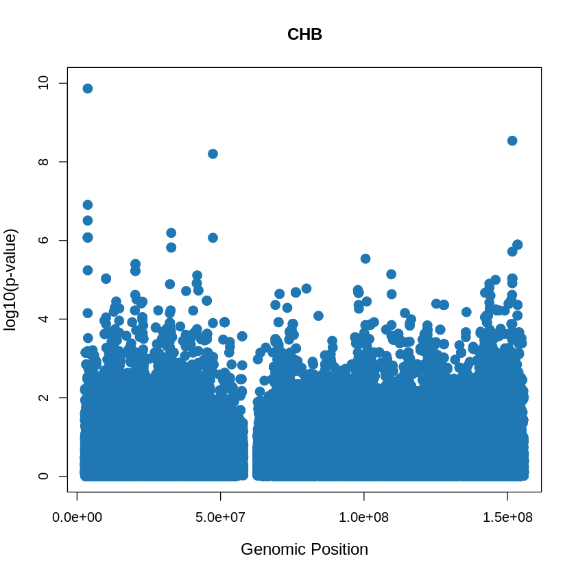
CHB <- read.table("/home/ari/ari-intern/people/ari/ariadna-intern/steps/CHB/relate/run_relate/1000g_ppl_phased_haplotypes_selection.sele", header = TRUE)
head(CHB)

A data.frame: 6 × 35

	pos	rs_id	X3571428.500000	X357142.937500	X257030.656250	X184981.281250	X133128.375000	X95810.585938	X68953.507812	X49624.847656	⋯	X257.030640	X184.981262	X133.128357	X95.810577	X68.953499	X49.624844	X35.714287	X0.000000	when_DAF_is_half	when_mutation_has_freq2
	<int>	<chr>	<int>	<int>	<int>	<int>	<int>	<int>	<dbl>	<dbl>	⋯	<dbl>	<dbl>	<dbl>	<dbl>	<dbl>	<dbl>	<dbl>	<int>	<dbl>	<dbl>
1	2781927	.	1	1	1	1	1	1	1	1	⋯	-0.469389	-0.1350390	-0.0537125	-0.0683953	-0.1218410	-1.66876e-05	-4.30725e-07	0	-0.357821	-0.707989
2	2781986	.	1	1	1	1	1	1	1	1	⋯	-0.469389	-0.1350390	-0.0537125	-0.0683953	-0.1218410	-1.66876e-05	-4.30725e-07	0	-0.357821	-0.707989
3	2782161	.	1	1	1	1	1	1	1	1	⋯	-0.134001	-0.1969290	-0.3636970	-0.1665180	-0.0778992	-1.11767e-01	-1.29266e-06	0	-0.223143	-0.803470
4	2782572	.	1	1	1	1	1	1	1	1	⋯	-0.352616	-0.0748059	-0.0297824	-0.1350440	-0.0487577	0.00000e+00	0.00000e+00	0	-0.314035	-2.224800
5	2784758	.	1	1	1	1	1	1	1	1	⋯	-0.414356	-0.1018040	-0.1638560	-0.1877580	-0.0405383	-3.93919e-05	0.00000e+00	0	-0.292926	-0.067107
6	2784905	.	1	1	1	1	1	1	1	1	⋯	-0.414356	-0.1018040	-0.1638560	-0.1877580	-0.0405383	-3.93919e-05	0.00000e+00	0	-0.292926	-0.067107

CHB_plot <- plot(CHB$pos, -(CHB$when_mutation_has_freq2), pch = 19, col = "#1F78B4", xlab = "Genomic Position", ylab = "log10(p-value)", main = "CHB" , cex = 1.5, ylim = c(0, 10), cex.lab = 1.2)
pdf("CHB_plot.pdf", width = 20, height = 5)
CHB_plot <- plot(CHB$pos, -(CHB$when_mutation_has_freq2), 
                 pch = 19, col = "#1F78B4", 
                 xlab = "Genomic Position", 
                 ylab = "log10(p-value)", 
                 main = "CHB",
                 cex = 1.5, 
                 yaxp = c(0, 10, 5),
                 cex.lab = 1.3,
                 cex.main = 1.6,  # Adjust title size
                 cex.axis = 1.2)  # Adjust axis numbers size

dev.off()

png: 2

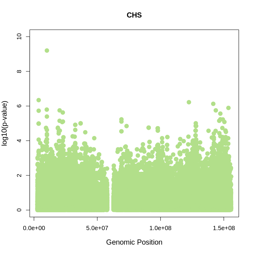
CHS <- read.table("/home/ari/ari-intern/people/ari/ariadna-intern/steps/CHS/relate/run_relate/1000g_ppl_phased_haplotypes_selection.sele", header = TRUE)
head(CHS)

A data.frame: 6 × 35

	pos	rs_id	X3571428.500000	X357142.937500	X257030.656250	X184981.281250	X133128.375000	X95810.585938	X68953.507812	X49624.847656	⋯	X257.030640	X184.981262	X133.128357	X95.810577	X68.953499	X49.624844	X35.714287	X0.000000	when_DAF_is_half	when_mutation_has_freq2
	<int>	<chr>	<int>	<int>	<int>	<int>	<int>	<int>	<int>	<dbl>	⋯	<dbl>	<dbl>	<dbl>	<dbl>	<dbl>	<dbl>	<dbl>	<int>	<dbl>	<dbl>
1	2781635	.	1	1	1	1	1	1	1	1	⋯	-0.509651	-0.5295390	-0.540640	-0.2382600	-0.353003	-0.495016	-0.453266	0	-0.6016760	-0.926999
2	2781927	.	1	1	1	1	1	1	1	1	⋯	-0.191600	-0.0350659	-0.102777	-0.0583544	-0.278356	-0.185307	-0.293794	0	-0.0503824	-0.294591
3	2781986	.	1	1	1	1	1	1	1	1	⋯	-0.191600	-0.0350659	-0.102777	-0.0583544	-0.278356	-0.185307	-0.293794	0	-0.0503824	-0.294591
4	2782161	.	1	1	1	1	1	1	1	1	⋯	-0.921153	-1.5332800	-0.849335	-0.7494320	-0.419384	-0.937000	-0.393215	0	-0.9510930	-1.741520
5	2782572	.	1	1	1	1	1	1	1	1	⋯	-0.719856	-0.7079780	-0.505628	-0.5949980	-0.269845	-0.588185	-0.232325	0	-0.5436550	-0.533548
6	2782784	.	1	1	1	1	1	1	1	1	⋯	1.000000	1.0000000	1.000000	1.0000000	1.000000	1.000000	1.000000	0	1.0000000	-0.701893

CHS_plot <- plot(CHS$pos, -(CHS$when_mutation_has_freq2), pch = 19, col = "#B2DF8A", xlab = "Genomic Position", ylab = "log10(p-value)", main = "CHS" , cex = 1.5, ylim = c(0, 10), cex.lab = 1.2)
pdf("CHS_plot.pdf", width = 20, height = 5)
CHS_plot <- plot(CHS$pos, -(CHS$when_mutation_has_freq2), 
                 pch = 19, col = "#B2DF8A", 
                 xlab = "Genomic Position", 
                 ylab = "log10(p-value)", 
                 main = "CHS",
                 cex = 1.5, 
                 yaxp = c(0, 10, 5),
                 cex.lab = 1.3,
                 cex.main = 1.6,  # Adjust title size
                 cex.axis = 1.2)  # Adjust axis numbers size

dev.off()

png: 2

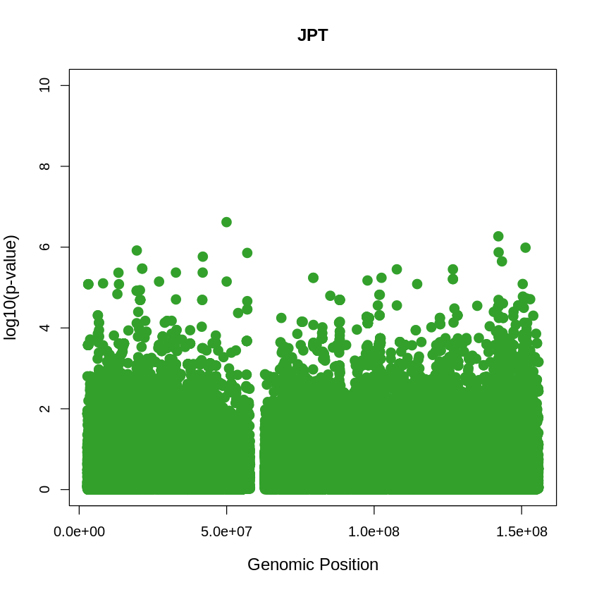
JPT <- read.table("/home/ari/ari-intern/people/ari/ariadna-intern/steps/JPT/relate/run_relate/1000g_ppl_phased_haplotypes_selection.sele", header = TRUE)
head(JPT)

A data.frame: 6 × 35

	pos	rs_id	X3571428.500000	X357142.937500	X257030.656250	X184981.281250	X133128.375000	X95810.585938	X68953.507812	X49624.847656	⋯	X257.030640	X184.981262	X133.128357	X95.810577	X68.953499	X49.624844	X35.714287	X0.000000	when_DAF_is_half	when_mutation_has_freq2
	<int>	<chr>	<int>	<int>	<int>	<int>	<int>	<int>	<dbl>	<dbl>	⋯	<dbl>	<dbl>	<dbl>	<dbl>	<dbl>	<dbl>	<dbl>	<int>	<dbl>	<dbl>
1	2781514	.	1	1	1	1	1	1	1	1	⋯	-0.544881	-0.543074	-0.3360220	-0.5822880	-0.4354700	-0.6970980	-1.1308500	0	-0.548842	-0.746704
2	2781986	.	1	1	1	1	1	1	1	1	⋯	-0.354544	-0.370605	-0.0512392	-0.0805736	-0.0537353	-0.1730980	-0.4372470	0	-0.455204	-0.112781
3	2782572	.	1	1	1	1	1	1	1	1	⋯	-0.319862	-0.318994	-0.4698040	-0.2719470	-0.0442616	-0.0408214	-0.0908543	0	-0.396086	-1.069260
4	2784758	.	1	1	1	1	1	1	1	1	⋯	-0.629078	-0.263415	-0.7430090	-0.3709640	-0.8436410	-0.9887650	-0.7396860	0	-0.796063	-0.483658
5	2784905	.	1	1	1	1	1	1	1	1	⋯	-0.629078	-0.263415	-0.7430090	-0.3709640	-0.8436410	-0.9887650	-0.7396860	0	-0.796063	-0.483658
6	2785313	.	1	1	1	1	1	1	1	1	⋯	-0.629078	-0.263415	-0.7430090	-0.3709640	-0.8436410	-0.9887650	-0.7396860	0	-0.796063	-0.483658

JPT_plot <- plot(JPT$pos, -(JPT$when_mutation_has_freq2), pch = 19, col = "#33A02C", xlab = "Genomic Position", ylab = "log10(p-value)", main = "JPT" , cex = 1.5, ylim = c(0, 10), cex.lab = 1.2)
pdf("JPT_plot.pdf", width = 20, height = 5)
JPT_plot <- plot(JPT$pos, -(JPT$when_mutation_has_freq2), 
                 pch = 19, col = "#33A02C", 
                 xlab = "Genomic Position", 
                 ylab = "log10(p-value)", 
                 main = "JPT",
                 cex = 1.5, 
                 yaxp = c(0, 10, 5),
                 cex.lab = 1.3,
                 cex.main = 1.6,  # Adjust title size
                 cex.axis = 1.2)  # Adjust axis numbers size

dev.off()

png: 2

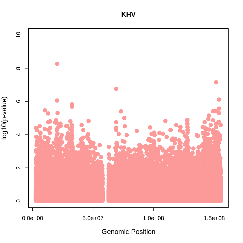
KHV <- read.table("/home/ari/ari-intern/people/ari/ariadna-intern/steps/KHV/relate/run_relate/1000g_ppl_phased_haplotypes_selection.sele", header = TRUE)
head(KHV)

A data.frame: 6 × 35

	pos	rs_id	X3571428.500000	X357142.937500	X257030.656250	X184981.281250	X133128.375000	X95810.585938	X68953.507812	X49624.847656	⋯	X257.030640	X184.981262	X133.128357	X95.810577	X68.953499	X49.624844	X35.714287	X0.000000	when_DAF_is_half	when_mutation_has_freq2
	<int>	<chr>	<int>	<int>	<int>	<int>	<int>	<int>	<dbl>	<dbl>	⋯	<dbl>	<dbl>	<dbl>	<dbl>	<dbl>	<dbl>	<dbl>	<int>	<dbl>	<dbl>
1	2781635	.	1	1	1	1	1	1	1	1	⋯	-0.8030350	-0.6989060	-0.605342	-0.45654000	-0.342867	-0.503979	-0.69663300	0	-1.0258700	-0.847264
2	2781927	.	1	1	1	1	1	1	1	1	⋯	-0.0590766	-0.0280912	-0.045688	-0.00312863	-0.010792	-0.018873	-0.00296262	0	-0.0553768	-0.635131
3	2781986	.	1	1	1	1	1	1	1	1	⋯	-0.0590766	-0.0280912	-0.045688	-0.00312863	-0.010792	-0.018873	-0.00296262	0	-0.0553768	-0.635131
4	2782161	.	1	1	1	1	1	1	1	1	⋯	-0.9175290	-1.2623400	-0.941499	-1.60266000	-1.237230	-1.025680	-1.11297000	0	-1.2013300	-0.406086
5	2784102	.	1	1	1	1	1	1	1	1	⋯	-1.3344400	-2.3292500	-1.154890	-1.79781000	-1.452120	-1.538880	-1.08854000	0	-2.0425200	-0.471176
6	2784738	.	1	1	1	1	1	1	1	1	⋯	1.0000000	1.0000000	1.000000	1.00000000	1.000000	1.000000	-0.56223200	0	-0.9722480	-0.418237

KHV_plot <- plot(KHV$pos, -(KHV$when_mutation_has_freq2), pch = 19, col = "#FB9A99", xlab = "Genomic Position", ylab = "log10(p-value)", main = "KHV" , cex = 1.5, ylim = c(0, 10), cex.lab = 1.2)
pdf("KHV_plot.pdf", width = 20, height = 5)
KHV_plot <- plot(KHV$pos, -(KHV$when_mutation_has_freq2), 
                 pch = 19, col = "#FB9A99", 
                 xlab = "Genomic Position", 
                 ylab = "log10(p-value)", 
                 main = "KHV",
                 cex = 1.5, 
                 yaxp = c(0, 10, 5),
                 cex.lab = 1.3,
                 cex.main = 1.6,  # Adjust title size
                 cex.axis = 1.2)  # Adjust axis numbers size

dev.off()

png: 2

library(wesanderson)
# Combine data frames
CDX$Population <- "CDX"
CHB$Population <- "CHB"
CHS$Population <- "CHS"
JPT$Population <- "JPT"
KHV$Population <- "KHV"

combined_data <- rbind(CDX, CHB, CHS, JPT, KHV)

custom_theme <- theme_minimal() +
  theme(
    text = element_text(size = 14),  # Increase the text size for all text elements
    plot.title = element_text(size = 16, hjust = 0.5),  # Increase the title size
    axis.title = element_text(size = 15),  # Increase the axis label size
    axis.text = element_text(size = 12),  # Increase the axis text size
    legend.text = element_text(size = 14)  # Increase the legend text size
  )

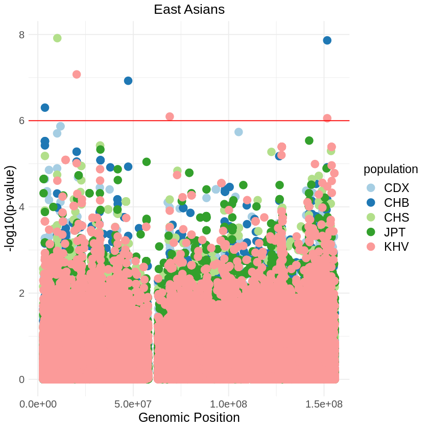
plot_combined <- ggplot(data = combined_data, aes(x = pos, y = -(when_mutation_has_freq2), color = Population)) +
  geom_point(pch = 19, size = 4) +
  labs(x = "Genomic Position", y = "log10(p-value)", title = "East Asians") +
  theme_light() + custom_theme +
  geom_hline(yintercept = 6, color = "red") +
  scale_color_brewer(palette = "Paired") + 
  theme(text = element_text(size = 15))

print(plot_combined)

ggsave("asians_threshold_REL_SQUARE.png", plot_combined, width = 7, height = 5)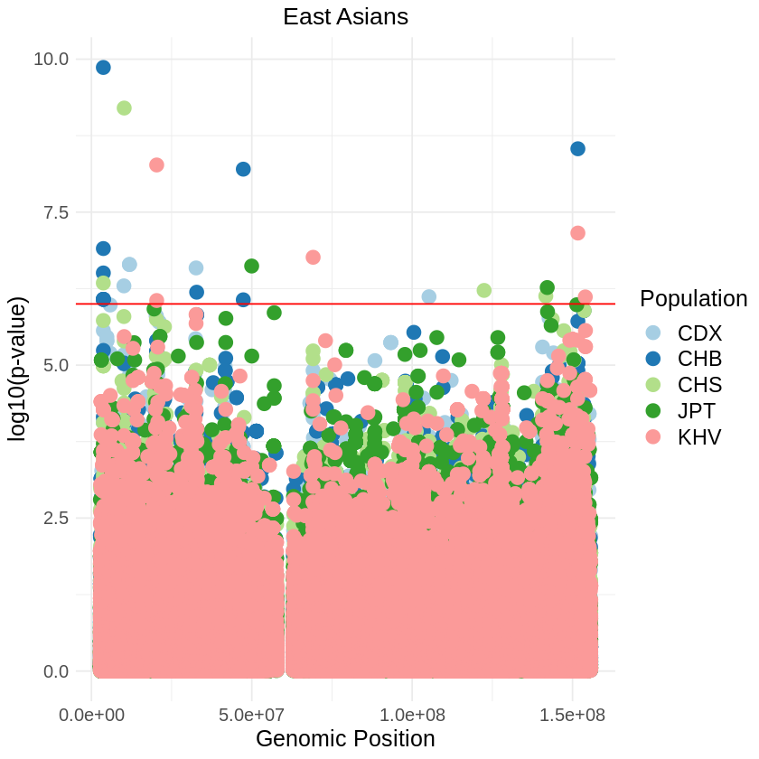

## SELECT JUST POSITION LOWER THAN THRESHOLD (log10 p-value < -6)

# Define file paths for the five .sele files
file_paths_asia <- c(
  "/home/ari/ari-intern/people/ari/ariadna-intern/steps/CDX/relate/run_relate/1000g_ppl_phased_haplotypes_selection.sele",
  "/home/ari/ari-intern/people/ari/ariadna-intern/steps/CHB/relate/run_relate/1000g_ppl_phased_haplotypes_selection.sele",
  "/home/ari/ari-intern/people/ari/ariadna-intern/steps/CHS/relate/run_relate/1000g_ppl_phased_haplotypes_selection.sele",
  "/home/ari/ari-intern/people/ari/ariadna-intern/steps/JPT/relate/run_relate/1000g_ppl_phased_haplotypes_selection.sele",
  "/home/ari/ari-intern/people/ari/ariadna-intern/steps/KHV/relate/run_relate/1000g_ppl_phased_haplotypes_selection.sele"
)

# Read the files
CDX <- read.table(file_paths_asia[1], header = TRUE)
CHB <- read.table(file_paths_asia[2], header = TRUE)
CHS <- read.table(file_paths_asia[3], header = TRUE)
JPT <- read.table(file_paths_asia[4], header = TRUE)
KHV <- read.table(file_paths_asia[5], header = TRUE)

# Function to subset data based on log10 p-value
subset_data <- function(data, population) {
  subset(data, when_mutation_has_freq2 < -6) %>%
    mutate(population = population)
}

# Define data frames and corresponding population names
file_pop <- list(
  list(data = CDX, population = "CDX"),
  list(data = CHB, population = "CHB"),
  list(data = CHS, population = "CHS"),
  list(data = JPT, population = "JPT"),
  list(data = KHV, population = "KHV")
)

# Subset and bind data from all files
asians_low_pvalue <- do.call(rbind, lapply(file_pop, function(fp) {
  subset_data(fp$data, fp$population)
}))

# Save the combined data to a single file
write.csv(asians_low_pvalue, "asians_low_pvalue.csv", row.names = FALSE)

filtered_asia <- read.csv("/home/ari/ari-intern/people/ari/ariadna-intern/notebooks/asians_low_pvalue.csv")
head(filtered_asia)
cat("Number of rows and columns:", paste(dim(filtered_asia), collapse = "x"))

A data.frame: 6 × 36

	pos	rs_id	X3571428.500000	X357142.937500	X257030.656250	X184981.281250	X133128.375000	X95810.585938	X68953.507812	X49624.847656	⋯	X184.981262	X133.128357	X95.810577	X68.953499	X49.624844	X35.714287	X0.000000	when_DAF_is_half	when_mutation_has_freq2	population
	<int>	<chr>	<int>	<int>	<int>	<int>	<int>	<int>	<int>	<int>	⋯	<dbl>	<dbl>	<dbl>	<dbl>	<dbl>	<dbl>	<int>	<dbl>	<dbl>	<chr>
1	10122953	.	1	1	1	1	1	1	1	1	⋯	-0.987813	-0.961790	-1.191430	-0.559613	-0.761888	-1.644260	0	-1.39061	-6.29509	CDX
2	11859476	.	1	1	1	1	1	1	1	1	⋯	-2.101280	-1.576190	-0.977768	-1.610050	-1.664170	-0.557903	0	-2.69332	-6.64483	CDX
3	11864438	.	1	1	1	1	1	1	1	1	⋯	-2.101280	-1.576190	-0.977768	-1.610050	-1.664170	-0.557903	0	-2.69332	-6.64483	CDX
4	32635171	.	1	1	1	1	1	1	1	1	⋯	-1.181500	-0.933064	-0.809430	-0.399554	-0.202704	-0.298736	0	-2.22411	-6.58804	CDX
5	105249963	.	1	1	1	1	1	1	1	1	⋯	-0.612386	-0.384370	-0.240353	-0.152790	-0.228024	-0.150998	0	-1.40614	-6.11750	CDX
6	3712725	.	1	1	1	1	1	1	1	1	⋯	-0.439584	-0.609713	-0.366916	-0.877111	-0.129806	0.000000	0	-1.08669	-6.50623	CHB

Number of rows and columns: 27x36

plot_threshold <- ggplot(filtered_asia, aes(x = pos, y = -(when_mutation_has_freq2), color = population)) +
  geom_point(size = 4) +
  labs(x = "Genomic position", y = "log10 p-value", title = "East Asian Populations") + 
  theme_minimal() + scale_color_brewer(palette = "Paired") + theme(text = element_text(size = 15),
        plot.title = element_text(hjust = 0.5))
print(plot_threshold)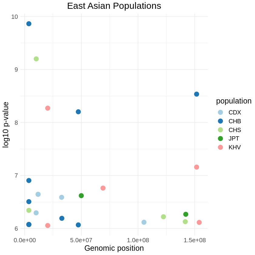

## PLOT TOGETHER ALL POPULATIONS SNPS BELOW THRESHOLD
# Define theme with larger text size for legend
custom_theme <- theme_minimal() +
  theme(
    text = element_text(size = 14),  # Increase the text size for all text elements
    plot.title = element_text(size = 16, hjust = 0.5),  # Increase the title size
    axis.title = element_text(size = 15),  # Increase the axis label size
    axis.text = element_text(size = 12),  # Increase the axis text size
    legend.text = element_text(size = 14)  # Increase the legend text size
  )

# Create plots with the custom theme
africa <- ggplot(filtered, aes(x = pos, y = -(when_mutation_has_freq2), color = population)) +
  geom_point(size = 6) +
  labs(x = NULL, y = NULL, title = "Africans") + 
  custom_theme +  # Apply the custom theme
  scale_color_brewer(palette = "Set2") + 
  ylim(6, 10)

europe <- ggplot(filtered_euro, aes(x = pos, y = -(when_mutation_has_freq2), color = population)) +
  geom_point(size = 6) +
  labs(x = NULL, y = NULL, title = "Europeans + PUR") + 
  custom_theme +  # Apply the custom theme
  scale_color_manual(values = c("GBR" = "lightblue", "FIN" = "lightpink", "IBS" = "gold", "TSI" = "lightgreen", "PUR" = "orange2")) +
  ylim(6, 10)

asia <- ggplot(filtered_asia, aes(x = pos, y = -(when_mutation_has_freq2), color = population)) +
  geom_point(size = 6) +
  labs(x = NULL, y = NULL, title = "East Asians") + 
  custom_theme +  # Apply the custom theme
  scale_color_manual(values = c("CDX" = "#A6CEE3", "CHB" = "#1F78B4", "CHS" = "#B2DF8A", "JPT" = "#33A02C", "KHV" = "#FB9A99")) + 
  ylim(6, 10)

# Combine the plots
combined_plots <- grid.arrange(africa, europe, asia, ncol = 1, 
                                left = "log10(p-value)",         
                                bottom = "Genomic position")

# Save the combined plot with larger text sizes
ggsave("combined_threshold_RELATE.png", combined_plots, width = 7, height = 15) 

Warning message:
“Removed 5 rows containing missing values (`geom_point()`).”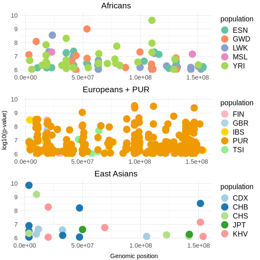

RUNS TEST

AFRICAN POPULATIONS

# Read the CSV files
LWK <- read.table("/home/ari/ari-intern/people/ari/ariadna-intern/steps/runs_test/1000g_ppl_phased_haplotypes_LWK_runstats.csv", sep=",", header=TRUE)
GWD <- read.table("/home/ari/ari-intern/people/ari/ariadna-intern/steps/runs_test/1000g_ppl_phased_haplotypes_GWD_runstats.csv", sep=",", header=TRUE)
ESN <- read.table("/home/ari/ari-intern/people/ari/ariadna-intern/steps/runs_test/1000g_ppl_phased_haplotypes_ESN_runstats.csv", sep=",", header=TRUE)
MSL <- read.table("/home/ari/ari-intern/people/ari/ariadna-intern/steps/runs_test/1000g_ppl_phased_haplotypes_MSL_runstats.csv", sep=",", header=TRUE)
YRI <- read.table("/home/ari/ari-intern/people/ari/ariadna-intern/steps/runs_test/1000g_ppl_phased_haplotypes_YRI_runstats.csv", sep=",", header=TRUE)

# Store the datasets in a list
datasets <- list(LWK=LWK, GWD=GWD, ESN=ESN, MSL=MSL, YRI=YRI)

# Loop over each dataset and modify them in place
for (name in names(datasets)) {
  # Get the dataset
  data <- datasets[[name]]
  
  # Filter the data
  filtered_data <- data %>%
    filter(stat_name == 'nr_runs' & nr_mut > 20)
  
  # Calculate -log10(p)
  filtered_data$log10p <- -log10(filtered_data$p)
  
  # Ensure 'stat' is treated as a factor
  filtered_data$stat <- as.factor(filtered_data$stat)
  
  # Assign the modified dataset back to the original variable name
  assign(name, filtered_data)
}

# Combine data frames
LWK$Population <- "LWK"
ESN$Population <- "ESN"
GWD$Population <- "GWD"
MSL$Population <- "MSL"
YRI$Population <- "YRI"

combined_data <- rbind(LWK, ESN, GWD, MSL, YRI)

custom_theme <- theme_minimal() +
  theme(
    text = element_text(size = 14),  # Increase the text size for all text elements
    plot.title = element_text(size = 16, hjust = 0.5),  # Increase the title size
    axis.title = element_text(size = 15),  # Increase the axis label size
    axis.text = element_text(size = 12),  # Increase the axis text size
    legend.text = element_text(size = 14)  # Increase the legend text size
  )

# Create the plot
plot_combined <- ggplot(data = combined_data, aes(x = pos, y = log10p, color = Population)) +
  geom_point(pch = 19, size = 4) +
  labs(x = "Genomic Position", y = "-log10(p-value)", title = "Africans") +
  theme_light() + custom_theme +
  geom_hline(yintercept = 6, color = "red") +
  scale_color_brewer(palette = "Set2") +
  theme(
    text = element_text(size = 15),
    plot.title = element_text(hjust = 0.5) # Center the title
  )

# Print the plot
print(plot_combined)
ggsave("africans_threshold_RUNS_SQUARE.png", plot_combined, width = 7, height = 5)

ERROR: Error: object 'stat_name' not found

Error: object 'stat_name' not found
Traceback:

1. data %>% filter(stat_name == "nr_runs" & nr_mut > 20)
2. filter(., stat_name == "nr_runs" & nr_mut > 20)

# Load necessary libraries
library(dplyr)
library(ggplot2)

# Define the file paths
file_paths <- list(
  LWK = "/home/ari/ari-intern/people/ari/ariadna-intern/steps/runs_test/1000g_ppl_phased_haplotypes_LWK_runstats.csv",
  GWD = "/home/ari/ari-intern/people/ari/ariadna-intern/steps/runs_test/1000g_ppl_phased_haplotypes_GWD_runstats.csv",
  ESN = "/home/ari/ari-intern/people/ari/ariadna-intern/steps/runs_test/1000g_ppl_phased_haplotypes_ESN_runstats.csv",
  MSL = "/home/ari/ari-intern/people/ari/ariadna-intern/steps/runs_test/1000g_ppl_phased_haplotypes_MSL_runstats.csv",
  YRI = "/home/ari/ari-intern/people/ari/ariadna-intern/steps/runs_test/1000g_ppl_phased_haplotypes_YRI_runstats.csv"
)

# Read the CSV files
datasets <- lapply(file_paths, function(path) {
  read.csv(path, stringsAsFactors = FALSE)
})

# Filter and process each dataset
datasets <- lapply(datasets, function(data) {
  data %>%
    filter(stat_name == 'nr_runs' & nr_mut > 20) %>%
    mutate(
      log10p = -log10(p),
      stat = as.factor(stat)
    )
})

# Combine data frames and add Population column
populations <- names(datasets)
for (i in seq_along(datasets)) {
  datasets[[i]]$Population <- populations[i]
}
combined_data <- do.call(rbind, datasets)

# Define the custom theme
custom_theme <- theme_minimal() +
  theme(
    text = element_text(size = 14),  # Increase the text size for all text elements
    plot.title = element_text(size = 16, hjust = 0.5),  # Increase the title size
    axis.title = element_text(size = 15),  # Increase the axis label size
    axis.text = element_text(size = 12),  # Increase the axis text size
    legend.text = element_text(size = 14)  # Increase the legend text size
  )

# Create the plot
plot_combined <- ggplot(data = combined_data, aes(x = pos, y = log10p, color = Population)) +
  geom_point(pch = 19, size = 4) +
  labs(x = "Genomic Position", y = "-log10(p-value)", title = "Africans") +
  theme_light() + custom_theme +
  geom_hline(yintercept = 6, color = "red") +
  scale_color_brewer(palette = "Set2") +
  theme(
    text = element_text(size = 15),
    plot.title = element_text(hjust = 0.5) # Center the title
  )

# Print the plot
print(plot_combined)
ggsave("africans_threshold_RUNS_SQUARE.png", plot_combined, width = 7, height = 5)

Attaching package: ‘dplyr’


The following object is masked from ‘package:gridExtra’:

    combine


The following objects are masked from ‘package:stats’:

    filter, lag


The following objects are masked from ‘package:base’:

    intersect, setdiff, setequal, union


Warning message:
“Removed 2353 rows containing missing values (`geom_point()`).”
Warning message:
“Removed 2353 rows containing missing values (`geom_point()`).”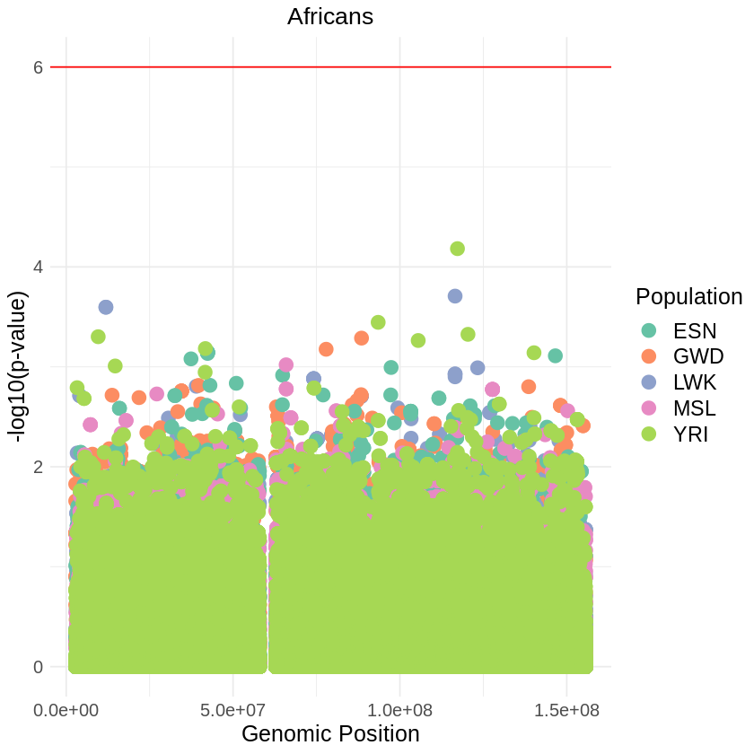

EUROPEANS + PUR

# Read the CSV files
GBR <- read.table("/home/ari/ari-intern/people/ari/ariadna-intern/steps/runs_test/1000g_ppl_phased_haplotypes_GBR_runstats.csv", sep=",", header=TRUE)
FIN <- read.table("/home/ari/ari-intern/people/ari/ariadna-intern/steps/runs_test/1000g_ppl_phased_haplotypes_FIN_runstats.csv", sep=",", header=TRUE)
IBS <- read.table("/home/ari/ari-intern/people/ari/ariadna-intern/steps/runs_test/1000g_ppl_phased_haplotypes_IBS_runstats.csv", sep=",", header=TRUE)
TSI <- read.table("/home/ari/ari-intern/people/ari/ariadna-intern/steps/runs_test/1000g_ppl_phased_haplotypes_TSI_runstats.csv", sep=",", header=TRUE)
PUR <- read.table("/home/ari/ari-intern/people/ari/ariadna-intern/steps/runs_test/1000g_ppl_phased_haplotypes_PUR_runstats.csv", sep=",", header=TRUE)

# Store the datasets in a list
datasets <- list(GBR=GBR, FIN=FIN, IBS=IBS, TSI=TSI, PUR=PUR)

# Loop over each dataset and modify them in place
for (name in names(datasets)) {
  # Get the dataset
  data <- datasets[[name]]
  
  # Filter the data
  filtered_data <- data %>%
    filter(stat_name == 'nr_runs' & nr_mut > 20)
  
  # Calculate -log10(p)
  filtered_data$log10p <- -log10(filtered_data$p)
  
  # Ensure 'stat' is treated as a factor
  filtered_data$stat <- as.factor(filtered_data$stat)
  
  # Assign the modified dataset back to the original variable name
  assign(name, filtered_data)
}

# Combine data frames
GBR$Population <- "GBR"
FIN$Population <- "FIN"
IBS$Population <- "IBS"
TSI$Population <- "TSI"
PUR$Population <- "PUR"

combined_data <- rbind(GBR, FIN, IBS, TSI, PUR)

custom_theme <- theme_minimal() +
  theme(
    text = element_text(size = 14),  # Increase the text size for all text elements
    plot.title = element_text(size = 16, hjust = 0.5),  # Increase the title size
    axis.title = element_text(size = 15),  # Increase the axis label size
    axis.text = element_text(size = 12),  # Increase the axis text size
    legend.text = element_text(size = 14)  # Increase the legend text size
  )

# Create the plot
plot_combined <- ggplot(data = combined_data, aes(x = pos, y = log10p, color = Population)) +
  geom_point(pch = 19, size = 4) +
  labs(x = "Genomic Position", y = "-log10(p-value)", title = "Europeans + PUR") +
  theme_light() + custom_theme +
  geom_hline(yintercept = 6, color = "red") +
  scale_color_manual(values = c("GBR" = "lightblue", "FIN" = "lightpink", "IBS" = "gold", "TSI" = "lightgreen", "PUR" = "orange2"))+
  theme(
    text = element_text(size = 15),
    plot.title = element_text(hjust = 0.5) # Center the title
  )

# Print the plot
print(plot_combined)

ggsave("europeans_threshold_RUNS_SQUARE.png", plot_combined, width = 7, height = 5)

Warning message:
“Removed 7004 rows containing missing values (`geom_point()`).”
Warning message:
“Removed 7004 rows containing missing values (`geom_point()`).”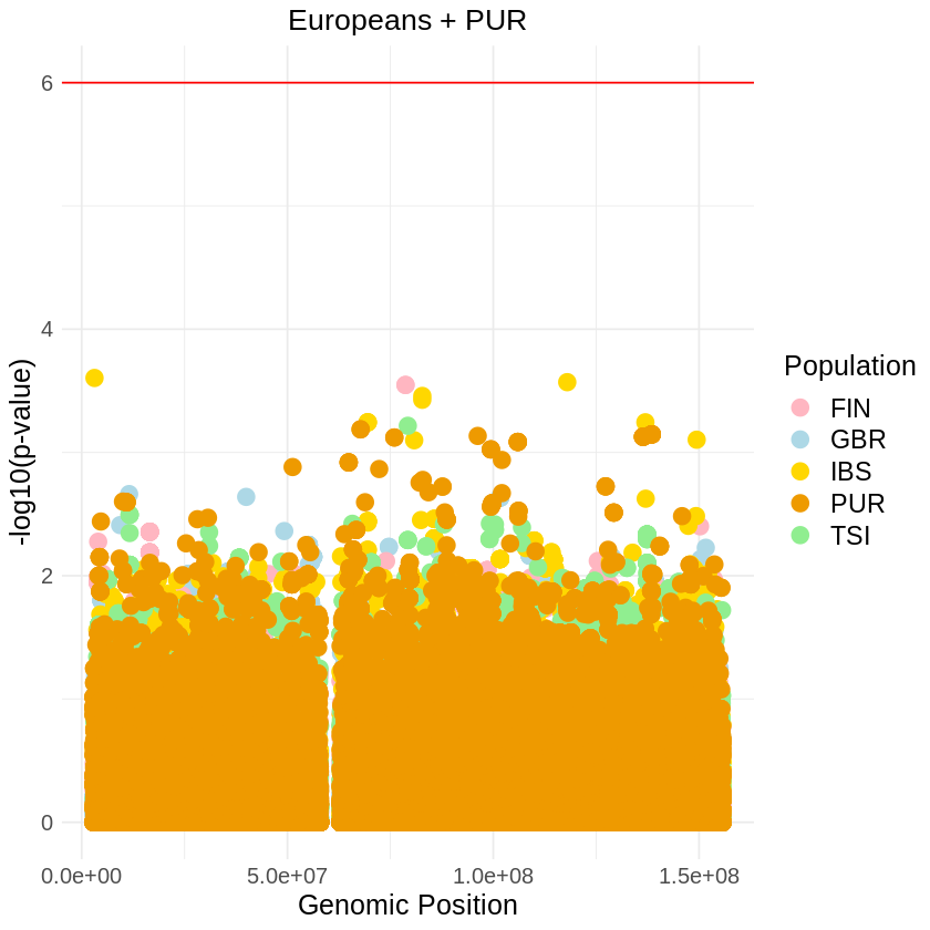

EAST ASIANS

# Load necessary library
library(dplyr)
library(ggplot2)

# Read the CSV files
CDX <- read.table("/home/ari/ari-intern/people/ari/ariadna-intern/steps/runs_test/1000g_ppl_phased_haplotypes_CDX_runstats.csv", sep=",", header=TRUE)
CHB <- read.table("/home/ari/ari-intern/people/ari/ariadna-intern/steps/runs_test/1000g_ppl_phased_haplotypes_CHB_runstats.csv", sep=",", header=TRUE)
CHS <- read.table("/home/ari/ari-intern/people/ari/ariadna-intern/steps/runs_test/1000g_ppl_phased_haplotypes_CHS_runstats.csv", sep=",", header=TRUE)
JPT <- read.table("/home/ari/ari-intern/people/ari/ariadna-intern/steps/runs_test/1000g_ppl_phased_haplotypes_JPT_runstats.csv", sep=",", header=TRUE)
KHV <- read.table("/home/ari/ari-intern/people/ari/ariadna-intern/steps/runs_test/1000g_ppl_phased_haplotypes_KHV_runstats.csv", sep=",", header=TRUE)

# Store the datasets in a list
datasets <- list(CDX=CDX, CHB=CHB, CHS=CHS, JPT=JPT, KHV=KHV)

# Loop over each dataset and modify them in place
for (name in names(datasets)) {
  # Get the dataset
  data <- datasets[[name]]
  
  # Filter the data
  filtered_data <- data %>%
    filter(stat_name == 'nr_runs' & nr_mut > 20)
  
  # Calculate -log10(p)
  filtered_data$log10p <- -log10(filtered_data$p)
  
  # Ensure 'stat' is treated as a factor
  filtered_data$stat <- as.factor(filtered_data$stat)
  
  # Assign the modified dataset back to the original variable name
  assign(name, filtered_data)
}

# Combine data frames
CDX$Population <- "CDX"
CHB$Population <- "CHB"
CHS$Population <- "CHS"
JPT$Population <- "JPT"
KHV$Population <- "KHV"

combined_data <- rbind(CDX, CHB, CHS, JPT, KHV)

custom_theme <- theme_minimal() +
  theme(
    text = element_text(size = 14),  # Increase the text size for all text elements
    plot.title = element_text(size = 16, hjust = 0.5),  # Increase the title size
    axis.title = element_text(size = 15),  # Increase the axis label size
    axis.text = element_text(size = 12),  # Increase the axis text size
    legend.text = element_text(size = 14)  # Increase the legend text size
  )

# Create the plot
plot_combined <- ggplot(data = combined_data, aes(x = pos, y = log10p, color = Population)) +
  geom_point(pch = 19, size = 4) +
  labs(x = "Genomic Position", y = "-log10(p-value)", title = "East Asians") +
  theme_light() + custom_theme +
  geom_hline(yintercept = 6, color = "red") +
  scale_color_brewer(palette = "Paired") +
  theme(
    text = element_text(size = 15),
    plot.title = element_text(hjust = 0.5) # Center the title
  )

# Print the plot
print(plot_combined)

ggsave("asians_threshold_RUNS_SQUARE_correct.png", plot_combined, width = 7, height = 5)

Warning message:
“Removed 5769 rows containing missing values (`geom_point()`).”
Warning message:
“Removed 5769 rows containing missing values (`geom_point()`).”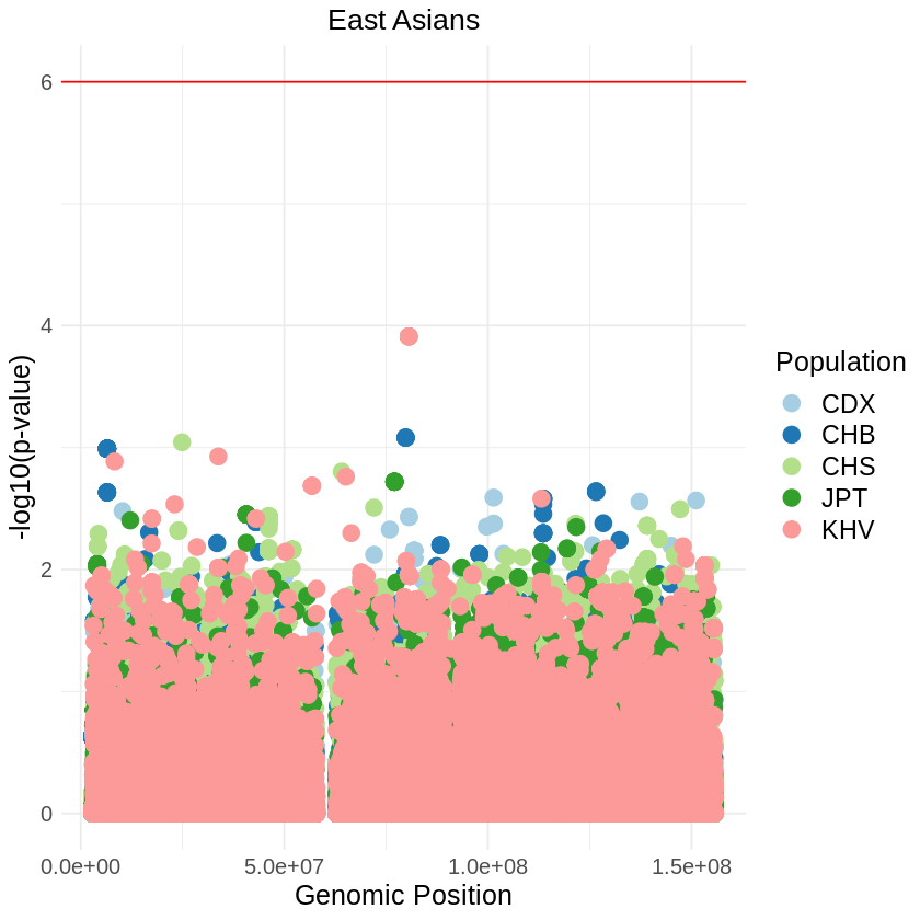

COMBINED P-VALUES

# Load the necessary library
library(dplyr)

# Define file paths for the five .sele files
file_paths_africa <- c(
  LWK = "/home/ari/ari-intern/people/ari/ariadna-intern/steps/fisher/combined_LWK.csv",
  ESN = "/home/ari/ari-intern/people/ari/ariadna-intern/steps/fisher/combined_ESN.csv",
  GWD = "/home/ari/ari-intern/people/ari/ariadna-intern/steps/fisher/combined_GWD.csv",
  MSL = "/home/ari/ari-intern/people/ari/ariadna-intern/steps/fisher/combined_MSL.csv",
  YRI = "/home/ari/ari-intern/people/ari/ariadna-intern/steps/fisher/combined_YRI.csv"
)

# Read the files
LWK <- read.csv(file_paths_africa["LWK"], header = TRUE)
ESN <- read.csv(file_paths_africa["ESN"], header = TRUE)
GWD <- read.csv(file_paths_africa["GWD"], header = TRUE)
MSL <- read.csv(file_paths_africa["MSL"], header = TRUE)
YRI <- read.csv(file_paths_africa["YRI"], header = TRUE)

# Function to subset data based on combined_p_values threshold
subset_data <- function(data, population) {
  data %>%
    filter(combined_p_values >= 6) %>%
    mutate(population = population)
}

# Define data frames and corresponding population names
file_pop <- list(
  list(data = LWK, population = "LWK"),
  list(data = ESN, population = "ESN"),
  list(data = GWD, population = "GWD"),
  list(data = MSL, population = "MSL"),
  list(data = YRI, population = "YRI")
)

# Subset and bind data from all files
africans_high_pvalue <- do.call(rbind, lapply(file_pop, function(fp) {
  subset_data(fp$data, fp$population)
}))

# Save the combined data to a single file
write.csv(africans_high_pvalue, "africans_combined.csv", row.names = FALSE)

Attaching package: ‘dplyr’


The following object is masked from ‘package:gridExtra’:

    combine


The following objects are masked from ‘package:stats’:

    filter, lag


The following objects are masked from ‘package:base’:

    intersect, setdiff, setequal, union

library(dplyr)
## SELECT JUST POSITION LOWER THAN THRESHOLD (log10 p-value < -6)
# Define file paths for the five .sele files
file_paths_euro <- c(
  "/home/ari/ari-intern/people/ari/ariadna-intern/steps/fisher/combined_GBR.csv",
  "/home/ari/ari-intern/people/ari/ariadna-intern/steps/fisher/combined_FIN.csv",
  "/home/ari/ari-intern/people/ari/ariadna-intern/steps/fisher/combined_IBS.csv",
  "/home/ari/ari-intern/people/ari/ariadna-intern/steps/fisher/combined_TSI.csv",
  "/home/ari/ari-intern/people/ari/ariadna-intern/steps/fisher/combined_PUR.csv"
)

# Read the files
GBR <- read.csv(file_paths_euro[1], header = TRUE)
FIN <- read.csv(file_paths_euro[2], header = TRUE)
IBS <- read.csv(file_paths_euro[3], header = TRUE)
TSI <- read.csv(file_paths_euro[4], header = TRUE)
PUR <- read.csv(file_paths_euro[5], header = TRUE)

# Function to subset data based on combined_p_values threshold
subset_data <- function(data, population) {
  data %>%
    filter(combined_p_values >= 6) %>%
    mutate(population = population)
}

# Define data frames and corresponding population names
file_pop <- list(
  list(data = GBR, population = "GBR"),
  list(data = FIN, population = "FIN"),
  list(data = IBS, population = "IBS"),
  list(data = TSI, population = "TSI"),
  list(data = PUR, population = "PUR")
)

# Subset and bind data from all files
europeans_low_pvalue <- do.call(rbind, lapply(file_pop, function(fp) {
  subset_data(fp$data, fp$population)
}))

# Save the combined data to a single file
write.csv(europeans_low_pvalue, "europeans_combined.csv", row.names = FALSE)

# Define file paths for the five .csv files
file_paths_asia_combined <- c(
  "/home/ari/ari-intern/people/ari/ariadna-intern/steps/fisher/combined_CDX.csv",
  "/home/ari/ari-intern/people/ari/ariadna-intern/steps/fisher/combined_CHB.csv",
  "/home/ari/ari-intern/people/ari/ariadna-intern/steps/fisher/combined_CHS.csv",
  "/home/ari/ari-intern/people/ari/ariadna-intern/steps/fisher/combined_JPT.csv",
  "/home/ari/ari-intern/people/ari/ariadna-intern/steps/fisher/combined_KHV.csv"
)

# Read the files
CDX <- read.csv(file_paths_asia_combined[1])
CHB <- read.csv(file_paths_asia_combined[2])
CHS <- read.csv(file_paths_asia_combined[3])
JPT <- read.csv(file_paths_asia_combined[4])
KHV <- read.csv(file_paths_asia_combined[5])

# Add population column to each data frame
CDX$population <- "CDX"
CHB$population <- "CHB"
CHS$population <- "CHS"
JPT$population <- "JPT"
KHV$population <- "KHV"

# Function to subset data based on combined_p_values
subset_data <- function(data, population) {
  data %>%
    filter(combined_p_values >= 6) %>%
    mutate(population = population)
}

# Define data frames and corresponding population names
file_pop <- list(
  list(data = CDX, population = "CDX"),
  list(data = CHB, population = "CHB"),
  list(data = CHS, population = "CHS"),
  list(data = JPT, population = "JPT"),
  list(data = KHV, population = "KHV")
)

# Subset and bind data from all files
asians_combined <- do.call(rbind, lapply(file_pop, function(fp) {
  subset_data(fp$data, fp$population)
}))

# Save the combined data to a single CSV file
write.csv(asians_combined, "asians_combined.csv", row.names = FALSE)

africa_file <- read.csv("/home/ari/ari-intern/people/ari/ariadna-intern/notebooks/africans_combined.csv")
europe_file <- read.csv("/home/ari/ari-intern/people/ari/ariadna-intern/notebooks/europeans_combined.csv")
asia_file <- read.csv("/home/ari/ari-intern/people/ari/ariadna-intern/notebooks/asians_combined.csv")

# Define theme with larger text size for legend
custom_theme <- theme_minimal() +
  theme(
    text = element_text(size = 14),  # Increase the text size for all text elements
    plot.title = element_text(size = 16, hjust = 0.5),  # Increase the title size
    axis.title = element_text(size = 15),  # Increase the axis label size
    axis.text = element_text(size = 12),  # Increase the axis text size
    legend.text = element_text(size = 14)  # Increase the legend text size
  )

# Create plots with the custom theme
africa <- ggplot(africa_file, aes(x = pos, y = (combined_p_values), color = population)) +
  geom_point(size = 6) +
  labs(x = NULL, y = NULL, title = "Africans") + 
  custom_theme +  # Apply the custom theme
  scale_color_brewer(palette = "Set2") + 
  ylim(6, 10)

europe <- ggplot(europe_file, aes(x = pos, y = (combined_p_values), color = population)) +
  geom_point(size = 6) +
  labs(x = NULL, y = NULL, title = "Europeans + PUR") + 
  custom_theme +  # Apply the custom theme
  scale_color_manual(values = c("GBR" = "lightblue", "FIN" = "lightpink", "IBS" = "gold", "TSI" = "lightgreen", "PUR" = "orange2")) +
  ylim(6, 10)

asia <- ggplot(asia_file, aes(x = pos, y = (combined_p_values), color = population)) +
  geom_point(size = 6) +
  labs(x = NULL, y = NULL, title = "East Asians") + 
  custom_theme +  # Apply the custom theme
  scale_color_manual(values = c("CDX" = "#A6CEE3", "CHB" = "#1F78B4", "CHS" = "#B2DF8A", "JPT" = "#33A02C", "KHV" = "#FB9A99")) + 
  ylim(6, 10)

# Combine the plots
combined_plots <- grid.arrange(africa, europe, asia, ncol = 1, 
                                left = "log10(p-value)",         
                                bottom = "Genomic position")

# Save the combined plot with larger text sizes
ggsave("combined_threshold_COMBINED_gap.png", combined_plots, width = 7, height = 15) 

Warning message:
“Removed 3 rows containing missing values (`geom_point()`).”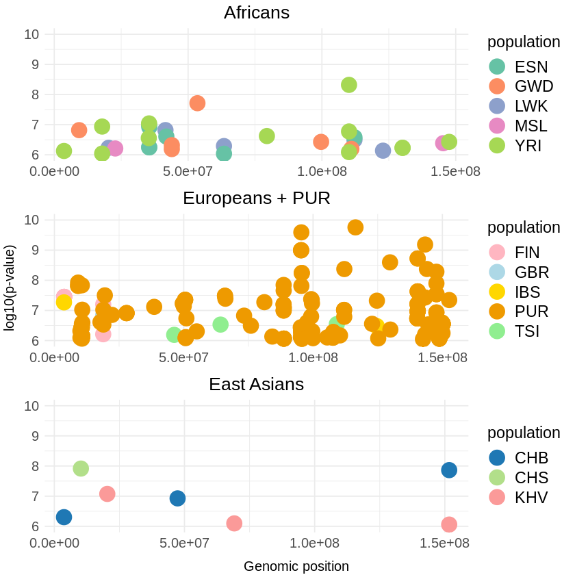

# Load the necessary libraries
library(dplyr)
library(ggplot2)

# Define file paths for the five .sele files
file_paths_africa <- c(
  LWK = "/home/ari/ari-intern/people/ari/ariadna-intern/steps/fisher/combined_LWK.csv",
  ESN = "/home/ari/ari-intern/people/ari/ariadna-intern/steps/fisher/combined_ESN.csv",
  GWD = "/home/ari/ari-intern/people/ari/ariadna-intern/steps/fisher/combined_GWD.csv",
  MSL = "/home/ari/ari-intern/people/ari/ariadna-intern/steps/fisher/combined_MSL.csv",
  YRI = "/home/ari/ari-intern/people/ari/ariadna-intern/steps/fisher/combined_YRI.csv"
)

# Read the files
LWK <- read.csv(file_paths_africa["LWK"], header = TRUE)
ESN <- read.csv(file_paths_africa["ESN"], header = TRUE)
GWD <- read.csv(file_paths_africa["GWD"], header = TRUE)
MSL <- read.csv(file_paths_africa["MSL"], header = TRUE)
YRI <- read.csv(file_paths_africa["YRI"], header = TRUE)

# Function to add population column to the data
add_population <- function(data, population) {
  data %>%
    mutate(population = population)
}

# Define data frames and corresponding population names
file_pop <- list(
  list(data = LWK, population = "LWK"),
  list(data = ESN, population = "ESN"),
  list(data = GWD, population = "GWD"),
  list(data = MSL, population = "MSL"),
  list(data = YRI, population = "YRI")
)

# Add population column and bind data from all files
africans_combined <- do.call(rbind, lapply(file_pop, function(fp) {
  add_population(fp$data, fp$population)
}))

# Save the combined data to a single file
write.csv(africans_combined, "africans_combined.csv", row.names = FALSE)

# Define theme with larger text size for legend
custom_theme <- theme_minimal() +
  theme(
    text = element_text(size = 14),  # Increase the text size for all text elements
    plot.title = element_text(size = 16, hjust = 0.5),  # Increase the title size
    axis.title = element_text(size = 15),  # Increase the axis label size
    axis.text = element_text(size = 12),  # Increase the axis text size
    legend.text = element_text(size = 14)  # Increase the legend text size
  )

# Create the plot
plot_combined <- ggplot(data = africans_combined, aes(x = pos, y = combined_p_values, color = population)) +
  geom_point(pch = 19, size = 4) +
  labs(x = "Genomic Position", y = "-log10(p-value)", title = "Africans") +
  theme_light() +
  custom_theme +
  scale_color_brewer(palette = "Set2") +
  geom_hline(yintercept = 6, color = "red")

# Print the plot
print(plot_combined)
ggsave("africans_combined_pvalues_SQUARE_big.png", plot_combined, width = 7, height = 5)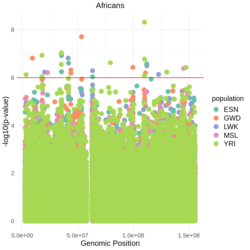

# Load the necessary libraries
library(dplyr)
library(ggplot2)

# Define file paths for the five .sele files
file_paths <- c(
  GBR = "/home/ari/ari-intern/people/ari/ariadna-intern/steps/fisher/combined_GBR.csv",
  FIN = "/home/ari/ari-intern/people/ari/ariadna-intern/steps/fisher/combined_FIN.csv",
  IBS = "/home/ari/ari-intern/people/ari/ariadna-intern/steps/fisher/combined_IBS.csv",
  TSI = "/home/ari/ari-intern/people/ari/ariadna-intern/steps/fisher/combined_TSI.csv",
  PUR = "/home/ari/ari-intern/people/ari/ariadna-intern/steps/fisher/combined_PUR.csv"
)

# Read the files
GBR <- read.csv(file_paths["GBR"], header = TRUE)
FIN <- read.csv(file_paths["FIN"], header = TRUE)
IBS <- read.csv(file_paths["IBS"], header = TRUE)
TSI <- read.csv(file_paths["TSI"], header = TRUE)
PUR <- read.csv(file_paths["PUR"], header = TRUE)

# Function to add population column to the data
add_population <- function(data, population) {
  data %>%
    mutate(population = population)
}

# Define data frames and corresponding population names
file_pop <- list(
  list(data = GBR, population = "GBR"),
  list(data = FIN, population = "FIN"),
  list(data = IBS, population = "IBS"),
  list(data = TSI, population = "TSI"),
  list(data = PUR, population = "PUR")
)

# Add population column and bind data from all files
combined_data <- do.call(rbind, lapply(file_pop, function(fp) {
  add_population(fp$data, fp$population)
}))

# Save the combined data to a single file
write.csv(combined_data, "european_populations.csv", row.names = FALSE)

# Create the plot
plot_combined <- ggplot(data = combined_data, aes(x = pos, y = combined_p_values, color = population)) +
  geom_point(pch = 19, size = 4) +
  labs(x = "Genomic Position", y = "-log10(p-value)", title = "Europeans+PUR") +
  theme_light() +
  custom_theme+
  scale_color_manual(values = c(
    "GBR" = "lightblue", 
    "FIN" = "lightpink", 
    "IBS" = "gold", 
    "TSI" = "lightgreen", 
    "PUR" = "orange2"
  )) +
  geom_hline(yintercept = 6, color = "red")

# Print the plot
print(plot_combined)
ggsave("europeans_combined_pvalues_SQUARE_big.png", plot_combined, width = 7, height = 5)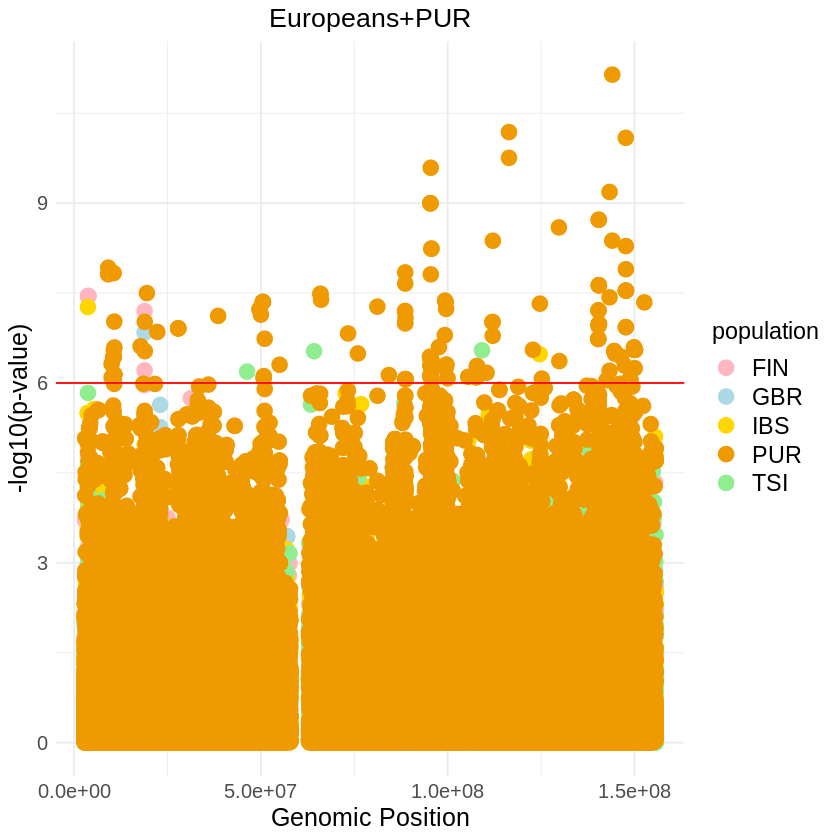

# Define file paths for the five .sele files
file_paths_asia <- c(
  CDX = "/home/ari/ari-intern/people/ari/ariadna-intern/steps/fisher/combined_CDX.csv",
  CHB = "/home/ari/ari-intern/people/ari/ariadna-intern/steps/fisher/combined_CHB.csv",
  CHS = "/home/ari/ari-intern/people/ari/ariadna-intern/steps/fisher/combined_CHS.csv",
  JPT = "/home/ari/ari-intern/people/ari/ariadna-intern/steps/fisher/combined_JPT.csv",
  KHV = "/home/ari/ari-intern/people/ari/ariadna-intern/steps/fisher/combined_KHV.csv"
)

# Read the files
CDX <- read.csv(file_paths_asia["CDX"], header = TRUE)
CHB <- read.csv(file_paths_asia["CHB"], header = TRUE)
CHS <- read.csv(file_paths_asia["CHS"], header = TRUE)
JPT <- read.csv(file_paths_asia["JPT"], header = TRUE)
KHV <- read.csv(file_paths_asia["KHV"], header = TRUE)

# Function to add population column to the data
add_population <- function(data, population) {
  data %>%
    mutate(population = population)
}

# Define data frames and corresponding population names
file_pop <- list(
  list(data = CDX, population = "CDX"),
  list(data = CHB, population = "CHB"),
  list(data = CHS, population = "CHS"),
  list(data = JPT, population = "JPT"),
  list(data = KHV, population = "KHV")
)

# Add population column and bind data from all files
asians_combined <- do.call(rbind, lapply(file_pop, function(fp) {
  add_population(fp$data, fp$population)
}))

# Save the combined data to a single file
write.csv(asians_combined, "asians_combined.csv", row.names = FALSE)

# Define theme with larger text size for legend
custom_theme <- theme_minimal() +
  theme(
    text = element_text(size = 14),  # Increase the text size for all text elements
    plot.title = element_text(size = 16, hjust = 0.5),  # Increase the title size
    axis.title = element_text(size = 15),  # Increase the axis label size
    axis.text = element_text(size = 12),  # Increase the axis text size
    legend.text = element_text(size = 14)  # Increase the legend text size
  )

# Create the plot
plot_combined <- ggplot(data = asians_combined, aes(x = pos, y = combined_p_values, color = population)) +
  geom_point(pch = 19, size = 4) +
  labs(x = "Genomic Position", y = "-log10(p-value)", title = "East Asians") +
  theme_light() +
  custom_theme +
  scale_color_brewer(palette = "Paired") +
  geom_hline(yintercept = 6, color = "red")

# Print the plot
print(plot_combined)
ggsave("asians_combined_pvalues_SQUARE_big.png", plot_combined, width = 7, height = 5)