Plots with matplotlib

import matplotlib.pyplot as plt
import seaborn as sns
sns.set_style("darkgrid")

# make graphics sharper on a good screen
from matplotlib_inline.backend_inline import set_matplotlib_formats
set_matplotlib_formats('retina', 'png')

plt.scatter(penguins.bill_length_mm, penguins.flipper_length_mm) ;  # semi colon makes last value None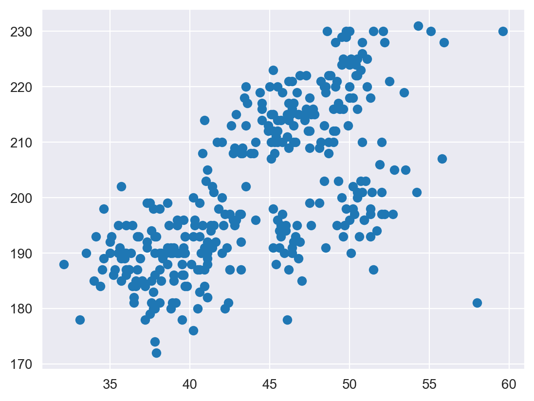

sns.set_style("ticks")
# sns.set_style("darkgrid")
# sns.set_style("whitegrid")
# sns.set_style("white")
# sns.set_style("dark")

plt.scatter(penguins.bill_length_mm, penguins.flipper_length_mm)
sns.despine()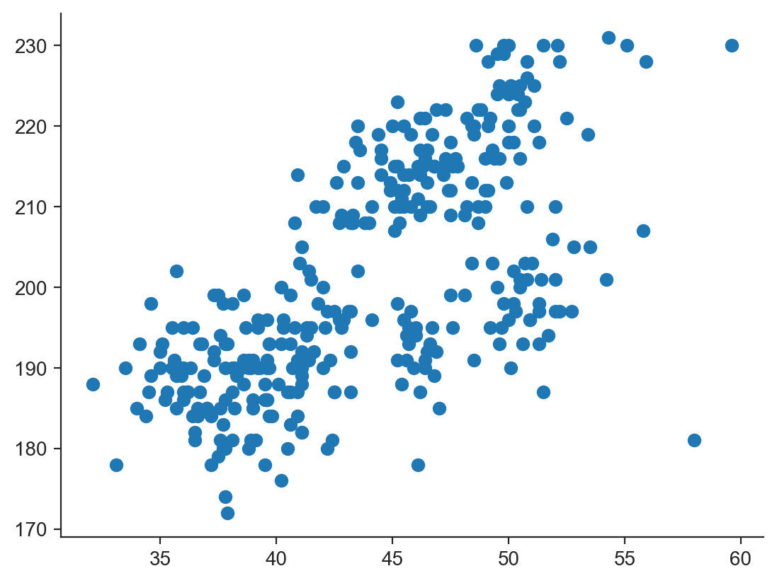

plt.hist(penguins.bill_length_mm) ;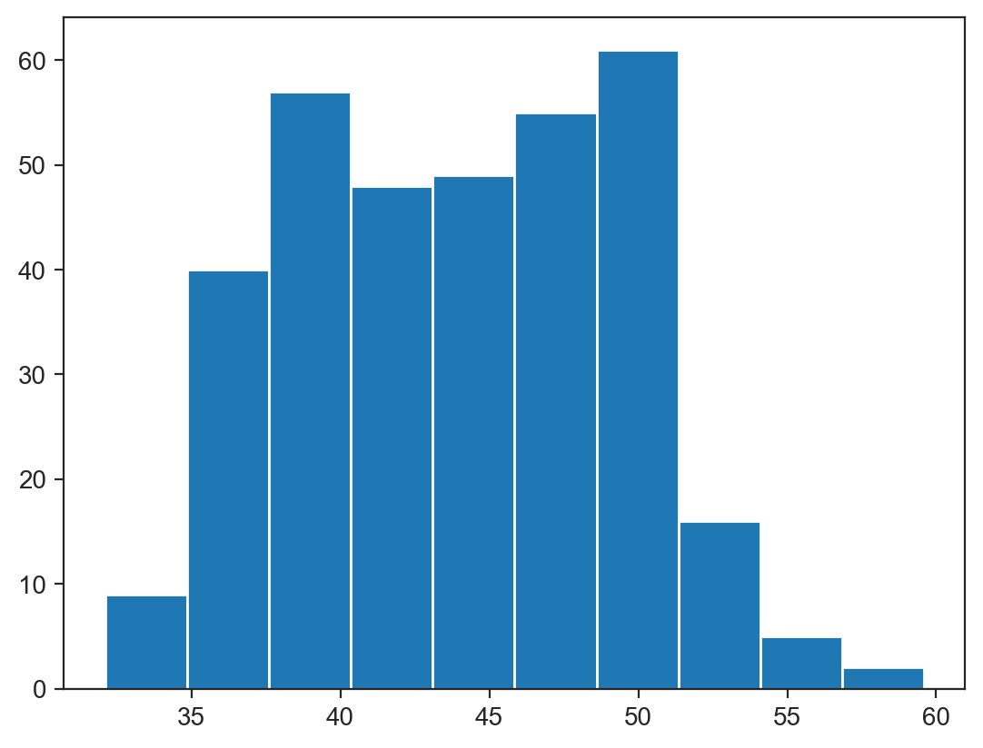

Better plotting with seaborn (on top of matplotlib)

sns.scatterplot(data=penguins, x="bill_length_mm", y="flipper_length_mm") ;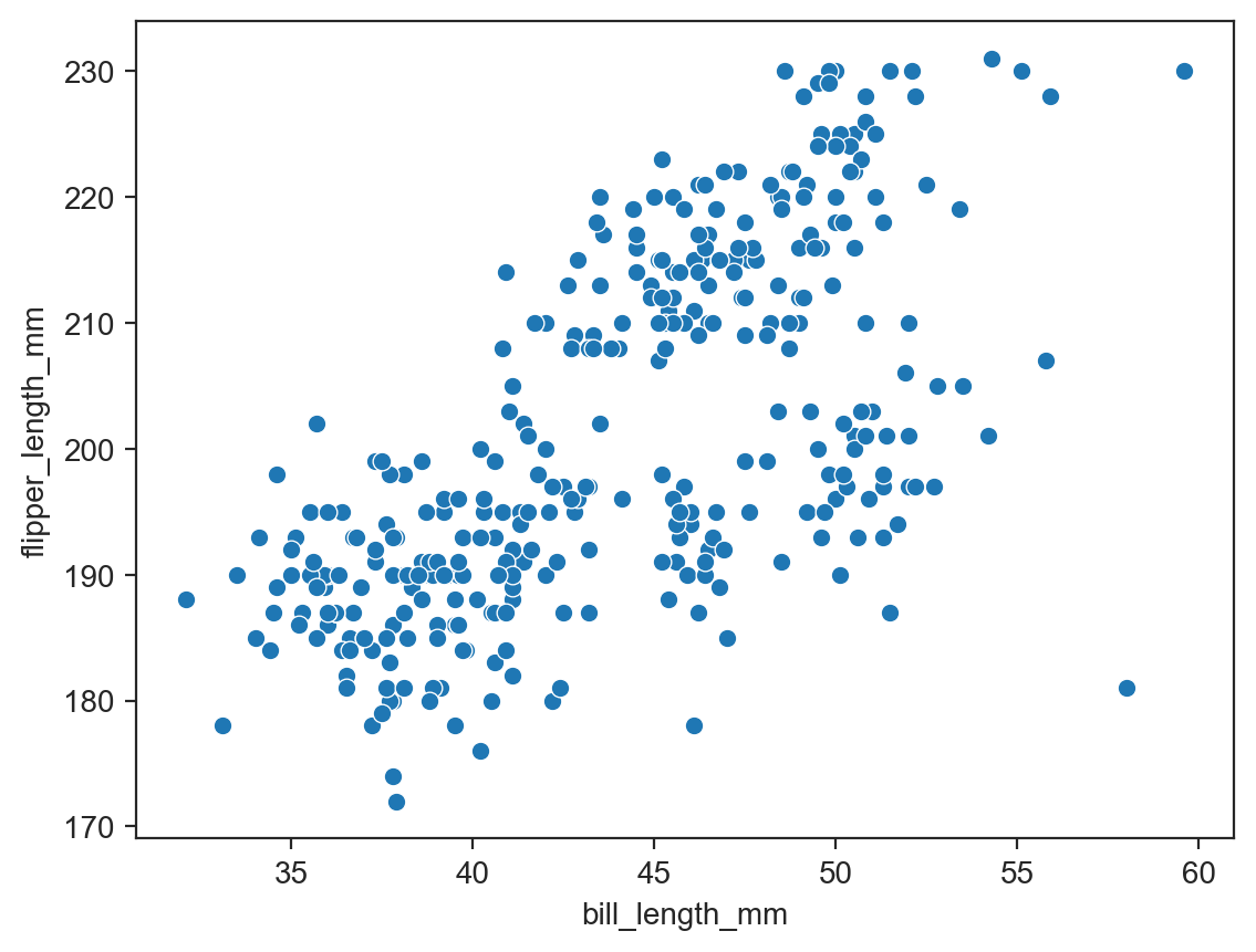

sns.scatterplot(data=penguins, x="bill_length_mm", y="flipper_length_mm", hue="species") ;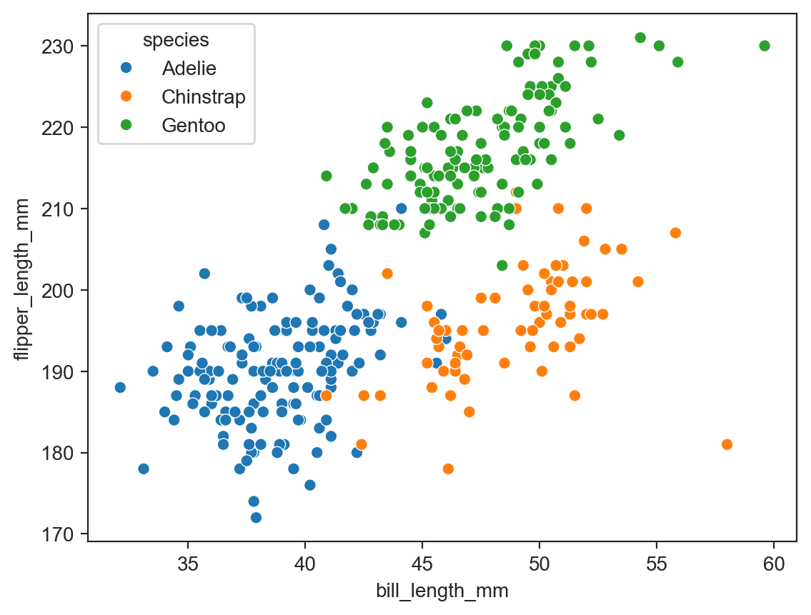

sns.scatterplot(data=penguins, x="bill_length_mm", y="flipper_length_mm", hue="species", style="sex") ;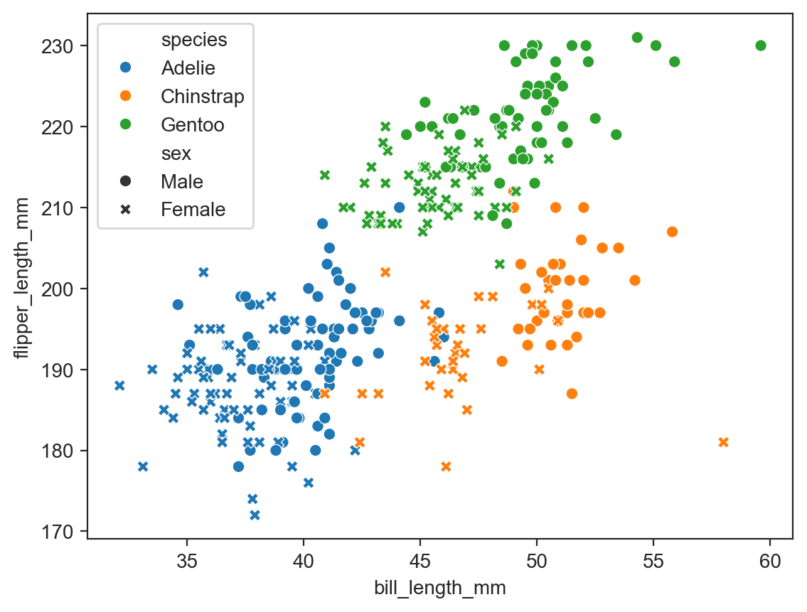

sns.scatterplot(data=penguins, x="bill_length_mm", y="flipper_length_mm", hue="species", 
                style="sex", size="body_mass_g") ;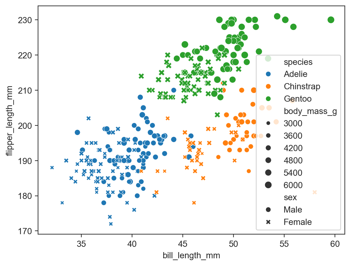

def legend_outside():
    plt.legend(bbox_to_anchor=(1.05, 1), loc='upper left', borderaxespad=0)

sns.scatterplot(data=penguins, x="bill_length_mm", y="flipper_length_mm", hue="species", style="sex", size="body_mass_g") ;

legend_outside()

plt.title("Penguin measurements")
plt.ylabel("flipper length (mm)")
plt.xlabel("bill length in (mm)") ;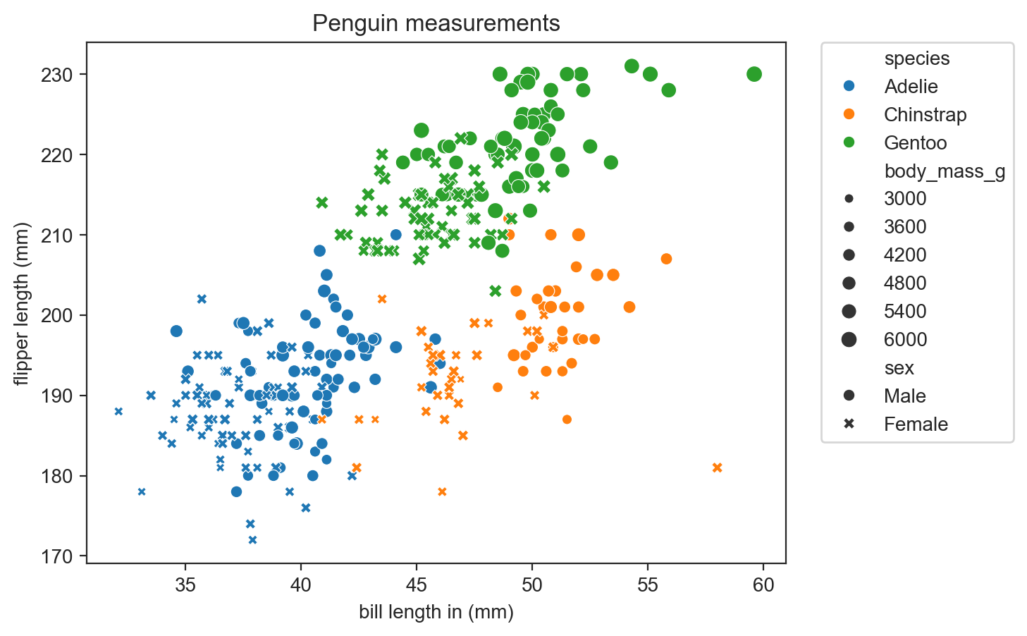

Wide or long data

Wide format data:

penguins[['bill_length_mm', 'bill_depth_mm']]

	bill_length_mm	bill_depth_mm
0	39.1	18.7
1	39.5	17.4
2	40.3	18.0
3	NaN	NaN
4	36.7	19.3
...	...	...
339	NaN	NaN
340	46.8	14.3
341	50.4	15.7
342	45.2	14.8
343	49.9	16.1

344 rows × 2 columns

Long format data:

long_df = penguins.melt(value_vars=['bill_length_mm', 'bill_depth_mm'])
long_df

	variable	value
0	bill_length_mm	39.1
1	bill_length_mm	39.5
2	bill_length_mm	40.3
3	bill_length_mm	NaN
4	bill_length_mm	36.7
...	...	...
683	bill_depth_mm	NaN
684	bill_depth_mm	14.3
685	bill_depth_mm	15.7
686	bill_depth_mm	14.8
687	bill_depth_mm	16.1

688 rows × 2 columns

long format is required when you want a number of columns to appear as a “variable” in the plot. As in the example below where the color “variable” reflects whether the point is bill_depth_mm or bill_length_mm.

Retain other information for each observation:

long_df = penguins.melt(id_vars=['species', 'body_mass_g', 'island'], value_vars=['bill_length_mm', 'bill_depth_mm'])
long_df

	species	body_mass_g	island	variable	value
0	Adelie	3750.0	Torgersen	bill_length_mm	39.1
1	Adelie	3800.0	Torgersen	bill_length_mm	39.5
2	Adelie	3250.0	Torgersen	bill_length_mm	40.3
3	Adelie	NaN	Torgersen	bill_length_mm	NaN
4	Adelie	3450.0	Torgersen	bill_length_mm	36.7
...	...	...	...	...	...
683	Gentoo	NaN	Biscoe	bill_depth_mm	NaN
684	Gentoo	4850.0	Biscoe	bill_depth_mm	14.3
685	Gentoo	5750.0	Biscoe	bill_depth_mm	15.7
686	Gentoo	5200.0	Biscoe	bill_depth_mm	14.8
687	Gentoo	5400.0	Biscoe	bill_depth_mm	16.1

688 rows × 5 columns

sns.scatterplot(data=long_df, x='body_mass_g', y='value', hue='variable', style='species')
legend_outside()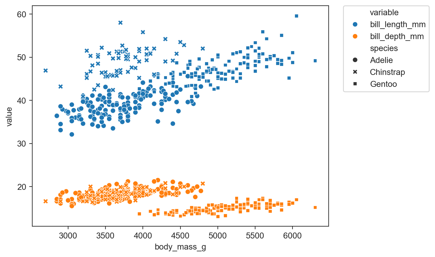

sns.boxplot(data=long_df, x='species', y='value', hue='variable') ;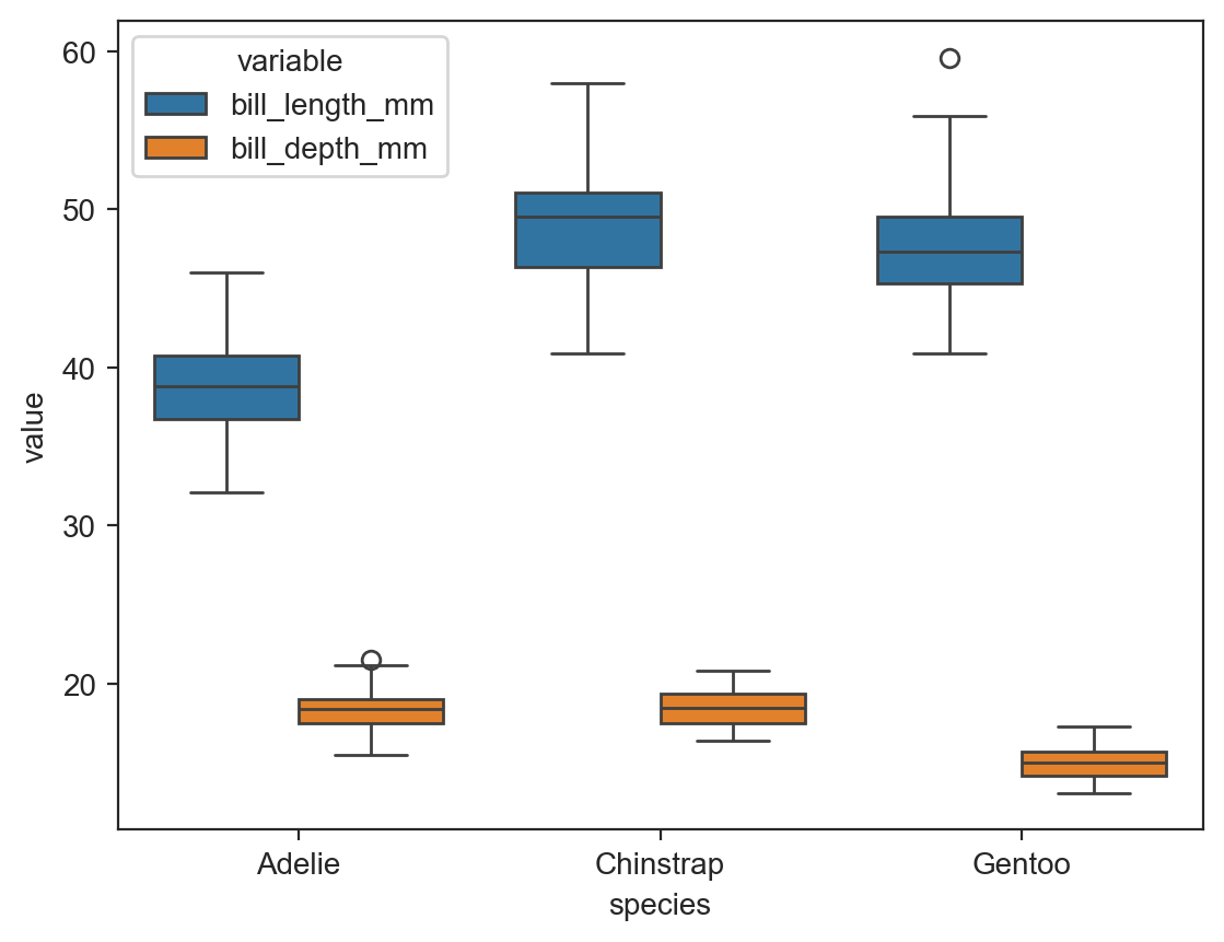

sns.boxplot(data=long_df, x='variable', y='value', hue='species') ;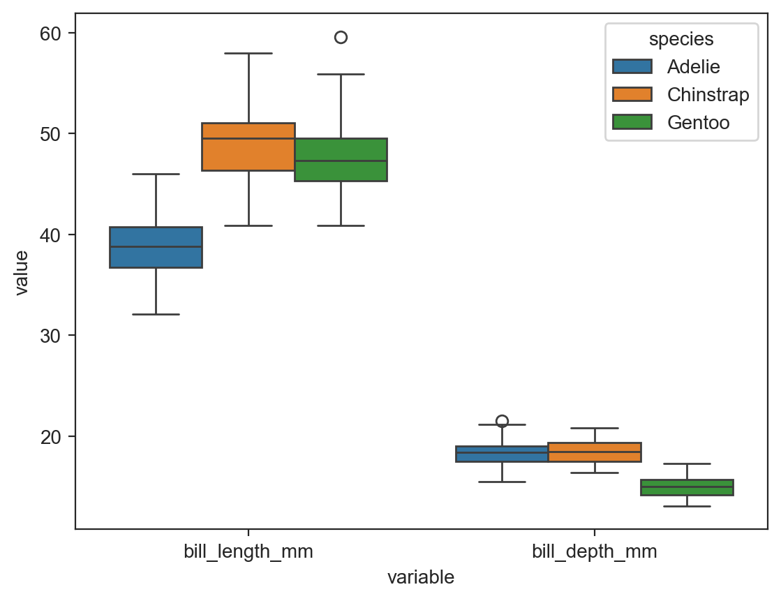

sns.boxplot(data=long_df, x='species', y='value', hue='variable') ;

Plots with multiple facets

g = sns.FacetGrid(penguins, col="island")
g ;

Map plotting to each facet:

g = sns.FacetGrid(penguins, col="island", hue="species") ;
g.map(sns.scatterplot, "bill_length_mm", "flipper_length_mm") ;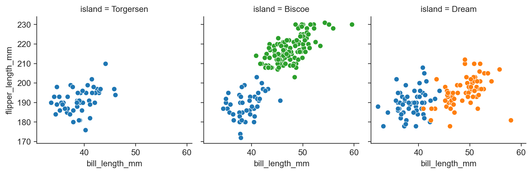

Grid of facets representing combinations of two variables:

g = sns.FacetGrid(penguins, row="sex", col="island", hue="species") ;
g.map(sns.scatterplot, "bill_length_mm", "flipper_length_mm") ;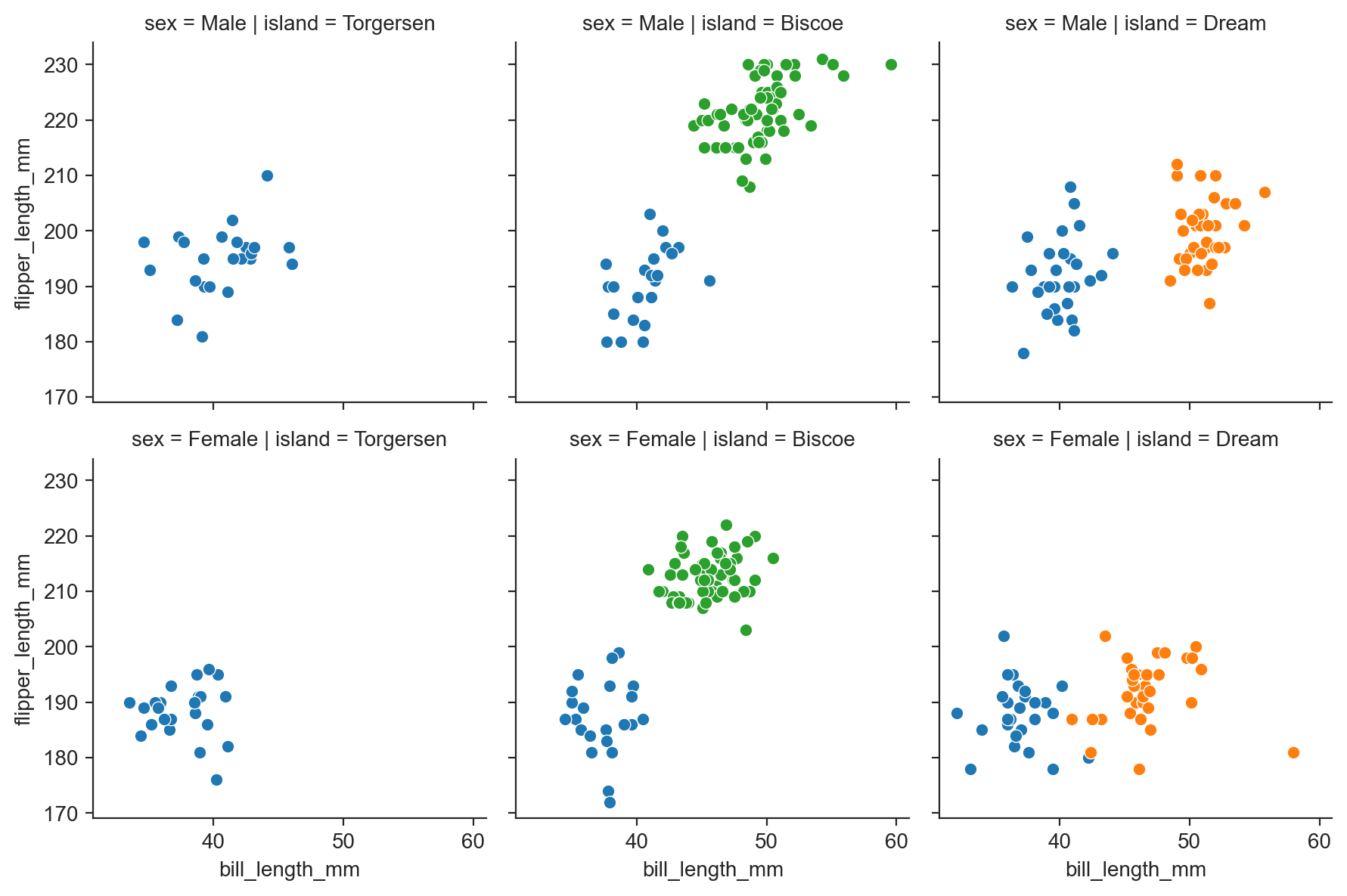

g = sns.FacetGrid(penguins, row="sex", col="island", hue="species") ;
g.map(sns.regplot, "bill_length_mm", "flipper_length_mm") ;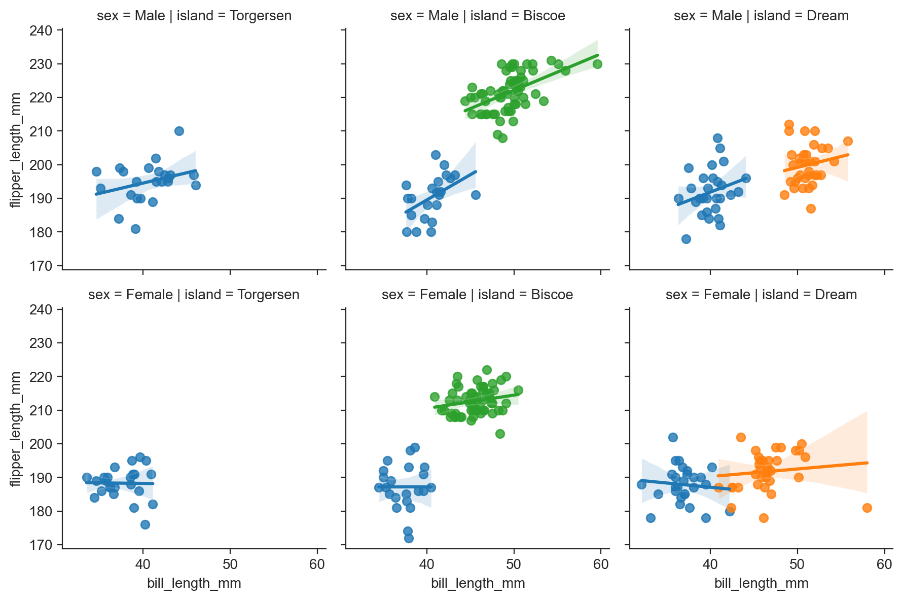

sns.lmplot(data=penguins, x="bill_length_mm", y="flipper_length_mm", row="sex", col="island", hue="species", height=3) ;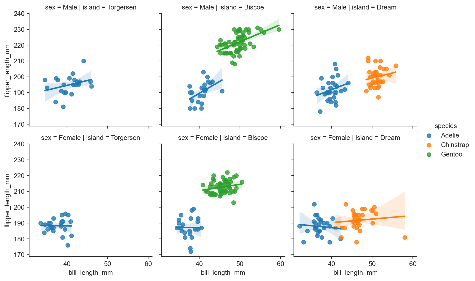

FacetGrid.map vs. FacetGrid.map_dataframe

When you use FacetGrid.map(func, "col1", "col2", ...), the function func is passed the values of the columns "col1" and "col2" (and more if needed) as parameters 1 and 2 (args[0], args[1], …). In addition, the function always receives a keyword argument named color=.

def scatter(*args, **kwargs):
    return plt.scatter(args[0], args[1], **kwargs)
    
g = sns.FacetGrid(penguins, row="sex", col="island", hue="species") ;
g.map(scatter, "bill_length_mm", "flipper_length_mm") ;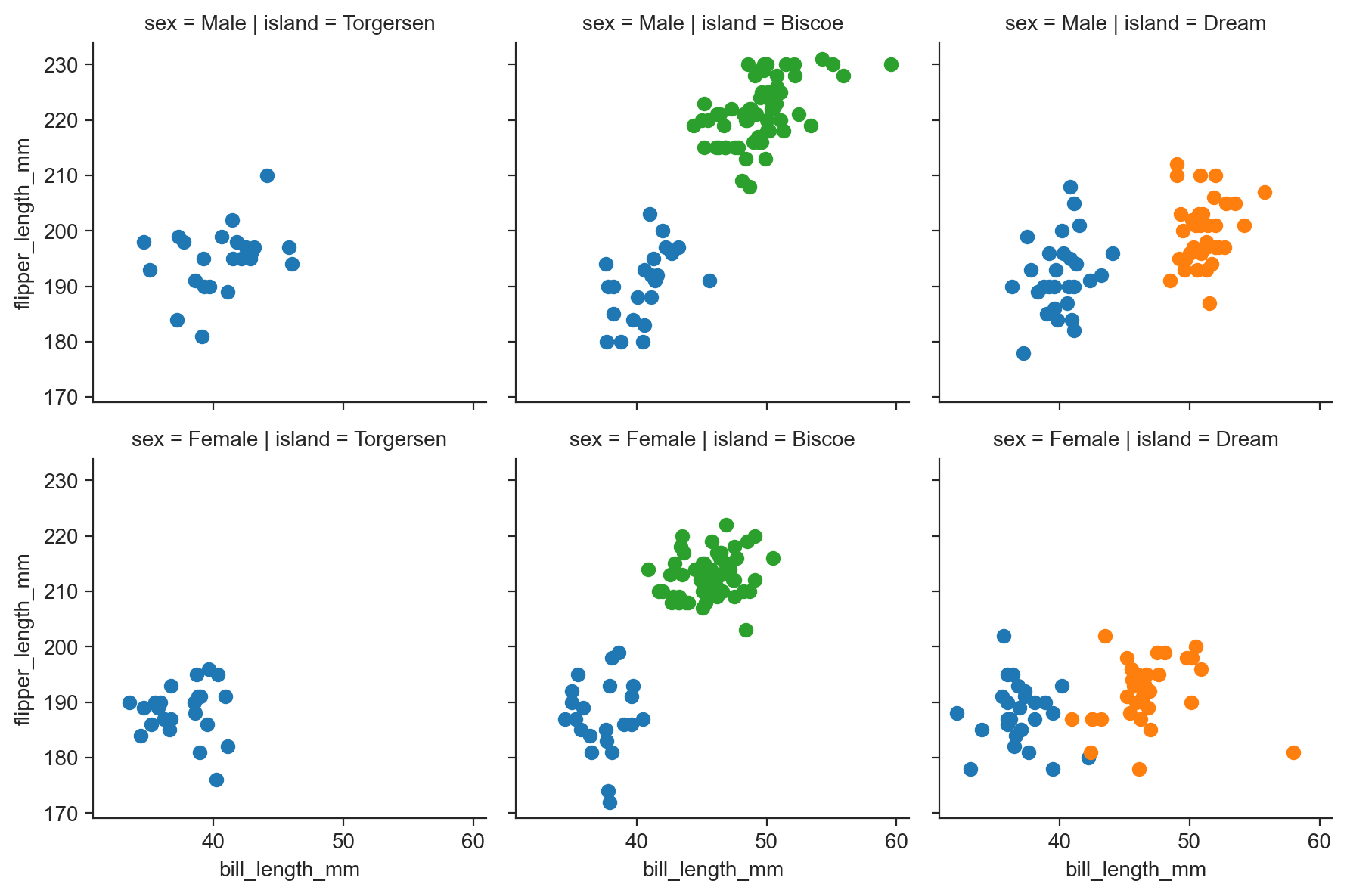

When you use FacetGrid.map_dataframe(func, "col1", "col2", ...), the function func is passed the names "col1" and "col2" (and more if needed) as parameters 1 and 2 (args[0], args[1], …), and the filtered dataframe as keyword argument data=. In addition, the function always receives a keyword argument named color=.

def scatterplot(*args, **kwargs):
    return sns.scatterplot(x=args[0], y=args[1], **kwargs)

g = sns.FacetGrid(penguins, row="sex", col="island", hue="species") ;
g.map_dataframe(scatterplot, "bill_length_mm", "flipper_length_mm") ;

g = sns.FacetGrid(penguins, row="sex", col="island", hue="species") ;
g.map(sns.histplot, "bill_length_mm") ;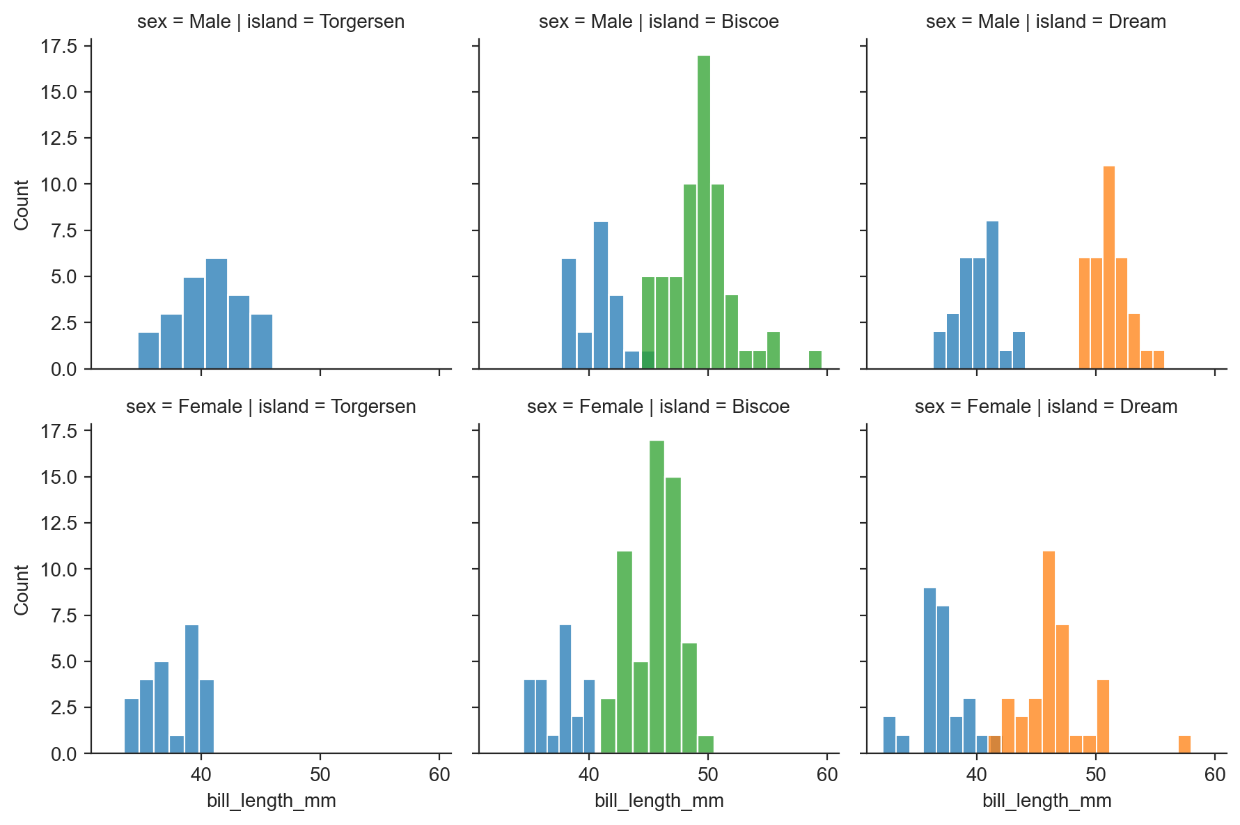

g = sns.FacetGrid(penguins, row="sex", col="island", hue="species") ;
g.map(sns.kdeplot, "bill_length_mm") ;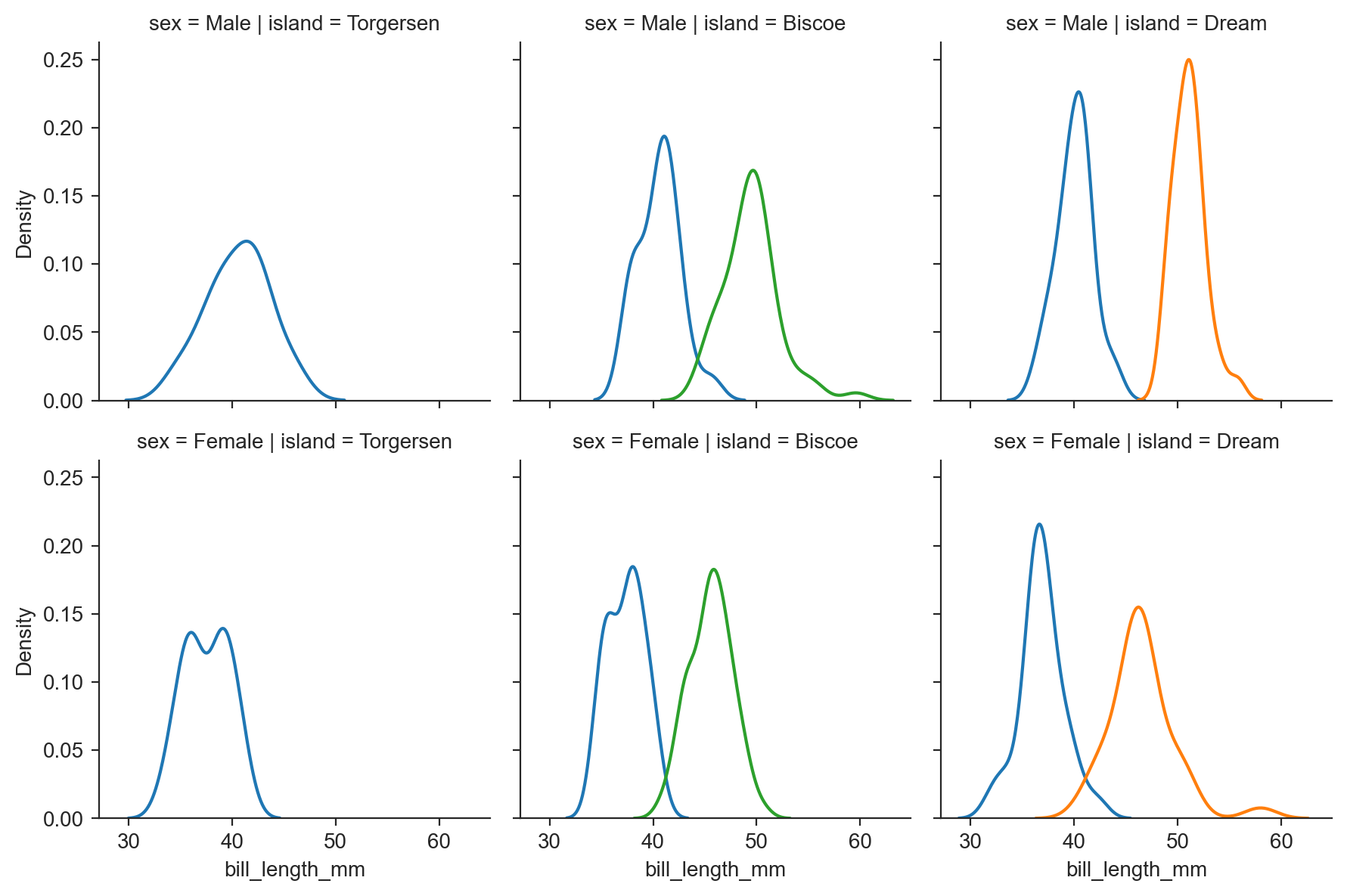

sns.pairplot(penguins, hue="species") ;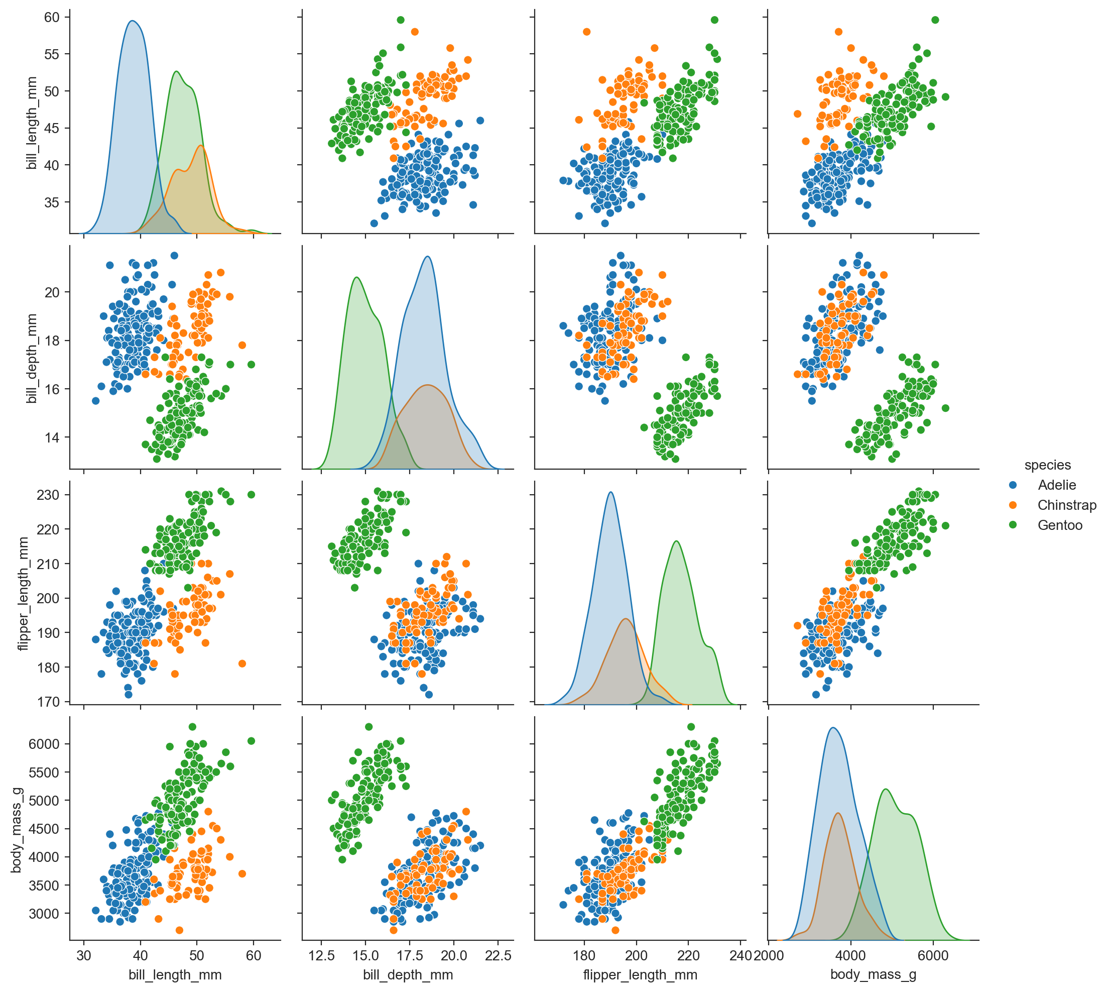

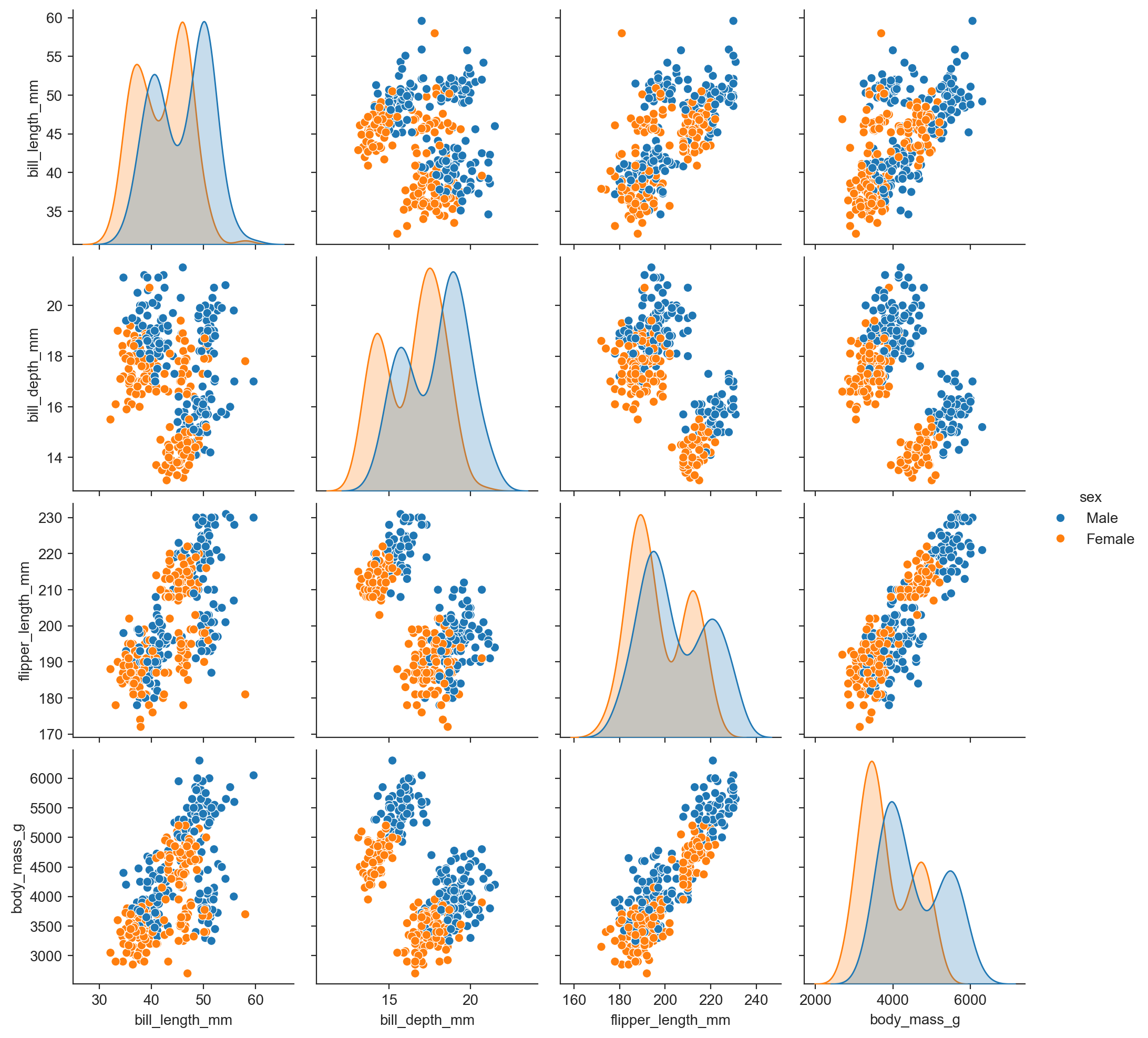
sns.pairplot(penguins, hue="sex") ;