import coolerimport pandas as pdimport glob%config InlineBackend.figure_format ='svg'
mclrs = glob.glob("../steps/cool/*/*.merged.mcool")clrs = [f"{mcl}::{res}"for mcl in mclrs for res in cooler.fileops.list_coolers(mcl)]# Locate the assembly reportreport ="../steps/ref/T2T-MMU8v1.0/assembly_report.txt"rep = pd.read_csv(report, sep="\t")length = rep[["Sequence-Length","Sequence-Name"]]rep_dict = rep.set_index("GenBank-Accn")["Sequence-Name"].to_dict()inv_dict = rep.set_index("Sequence-Name")["GenBank-Accn"].to_dict()for clr in clrs: tmp_clr = cooler.Cooler(clr) cooler.rename_chroms(tmp_clr, rep_dict)
Calculate the GC content
of the binned versions of the assembly (according to resolutions in mcool).
I will try to use the CLI to make quick work of it.
It is used as the phasing track for the eigendecomposition.
%%bash REF=../steps/ref/T2T-MMU8v1.0/T2T-MMU8v1.0.renamed.fafor res in100050001000050000100000; do BINS=../data/bins/t2tbins.${res}.tsv GC_OUT=../data/bins/gc.${res}.tsv cooltools genome gc $BINS $REF > $GC_OUTdone
Infer the centromeres
I found a T2T-MMU8v1repeatMasker.out.gz file and placed it ../steps/ref/T2T-MMU8v1/, then extracted information about longest stretches of satellite repeats.
%%bash # Navigatecd ../steps/ref/T2T-MMU8v1.0# Download repeatmasker output wget https://hgdownload.soe.ucsc.edu/hubs/GCA/049/350/105/GCA_049350105.1/GCA_049350105.1.repeatMasker.out.gz .# Find all the satellite repeats in the assemblyzcat GCA_049350105.1.repeatMasker.out.gz |\awk 'NR > 3 && $11 ~ /[Ss]atellite/ { print $5, $6-1, $7, $10 }' OFS='\t'> satellite_repeats.bed# Find the satellite repeats on chrXzcat GCA_049350105.1.repeatMasker.out.gz |\awk 'NR > 3 && $5 == "CM111679.1" && $11 ~ /[Ss]atellite/ { print $5, $6-1, $7, $10 }' OFS="\t"> chrX_satellites.bed# Merge the satellite repeats to find the centromerebedtools sort -i chrX_satellites.bed |\bedtools merge -d 20000-c 4-o distinct > chrX_centromere.bed# Find the largest satellite repeatawk '{ print $0, $3 - $2 }' chrX_centromere.bed | sort -k5,5nr| head -n1
chrom          CM111679.1
start            57984683
end              69396537
type      ALR/Alpha,HSAT4
length           11411854
Name: 8, dtype: object
Make a viewframe for cooltools
Here, we partition the chromosome into three parts. 1) small arm, 2) large arm, 3) centromere. The centromere is defined as the region of the chromosome that contains the longest stretch of satellite repeats.
%%bash # Find multires coolersMCOOLS=../steps/cool/*/*.merged.mcool# Define the viewframeVIEW=../data/view_T2T_MMU8v1_X_chromarms.tsvfor MCOOL in $MCOOLS; do# Get the tissue name TISSUE=$(basename $MCOOL .merged.mcool) echo $TISSUEfor res in100050001000050000100000; do COOLER=$MCOOL::resolutions/$res GC_BINS=../data/bins/gc.${res}.tsv EIGS_OUT=../data/eigs/$TISSUE.eigs.$res echo -ne ' -' $res OK cooltools eigs-cis -o $EIGS_OUT --view $VIEW --phasing-track $GC_BINS --n-eigs 3 $COOLER done echo ""doneecho All done
fibroblast
 - 1000 OK - 5000 OK - 10000 OK - 50000 OK - 100000 OK
pachytene_spermatocyte
 - 1000 OK - 5000 OK - 10000 OK - 50000 OK - 100000 OK
round_spermatid
 - 1000 OK - 5000 OK - 10000 OK - 50000 OK - 100000 OK
spermatogonia
 - 1000 OK - 5000 OK - 10000 OK - 50000 OK - 100000 OK
sperm
 - 1000 OK - 5000 OK - 10000 OK - 50000 OK - 100000 OK
All done
Check the results by eye
Define the eigenvectors
import pandas as pdfrom glob import globimport oseigfiles = glob("../data/eigs/*vecs.tsv")eignames = [os.path.basename(eig).split('.cis')[0] for eig in eigfiles]eignamesdf_eig = pd.DataFrame({'path': eigfiles,'tissue': [eigname.split('.eigs.')[0] for eigname in eignames],'resolution': [eigname.split('.eigs.')[1] for eigname in eignames]})
sperm_1000 = pd.read_csv(df_eig.query('tissue == "sperm" and resolution == "1000"')['path'].values[0], sep="\t", header=0)display(sperm_1000.head())sperm_dict = { res: pd.read_csv(df_eig.query('tissue == "sperm" and resolution == @res')['path'].values[0], sep="\t", header=0) for res in df_eig['resolution'].unique()}fib_dict = { res: pd.read_csv(df_eig.query('tissue == "fibroblast" and resolution == @res')['path'].values[0], sep="\t", header=0) for res in df_eig['resolution'].unique()}print(sperm_dict['1000'].head())
  chrom  start   end  weight  E1  E2  E3
0  chrX      0  1000     NaN NaN NaN NaN
1  chrX   1000  2000     NaN NaN NaN NaN
2  chrX   2000  3000     NaN NaN NaN NaN
3  chrX   3000  4000     NaN NaN NaN NaN
4  chrX   4000  5000     NaN NaN NaN NaN
chrom start end weight E1 E2 E3
0 chrX 0 1000 NaN NaN NaN NaN
1 chrX 1000 2000 NaN NaN NaN NaN
2 chrX 2000 3000 NaN NaN NaN NaN
3 chrX 3000 4000 NaN NaN NaN NaN
4 chrX 4000 5000 NaN NaN NaN NaN
import matplotlib.pyplot as pltimport numpy as np% config InlineBackend.figure_format ='retina'# Plot the E1 tracks saved in the sperm_dictdef plot_eigenvectors(eigenvectors, title=None): fig, ax = plt.subplots(figsize=(10, 2)) x = eigenvectors['start'] y = eigenvectors['E1'] ax.fill_between(x, y, where = y<0, color='tab:blue', lw=1, ec='None') ax.fill_between(x, y, where = y>0, color='tab:red', lw=1, ec='None') ax.set_title(title) ax.set_ylabel('E1') ax.set_xlim(x.min(), x.max()) ax.set_ylim(-1,1) ax.set_xlabel('Genomic Position (Mbp)') ticks = np.linspace(0, x.max(), num=10) ax.set_xticks(ticks) ax.set_xticklabels([f'{int(t/1e6)} Mbp'for t in ticks]) ax.spines[:].set_visible(False) ax.spines['bottom'].set_visible(True) fig.tight_layout()#res = '100000'#plot_eigenvectors(sperm_dict[res], title=f'Sperm E1 at {int(int(res)/1000)}kb resolution')
UsageError: Line magic function `%` not found.
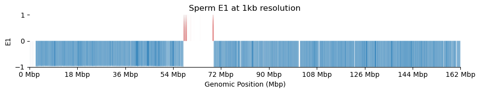
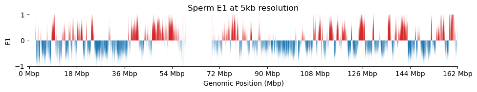
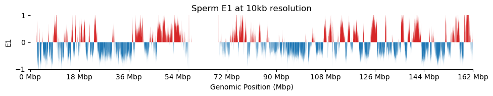
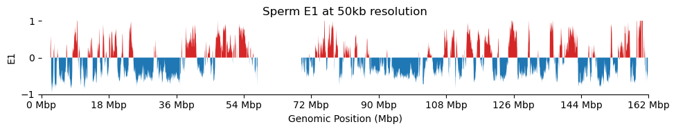
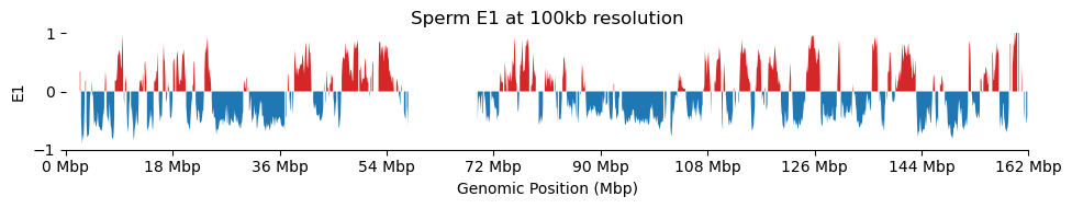
for res in ['1000', '5000', '10000', '50000', '100000']:
    plot_eigenvectors(sperm_dict[res], title=f'Sperm E1 at {int(int(res)/1000)}kb resolution')
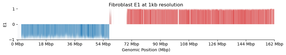
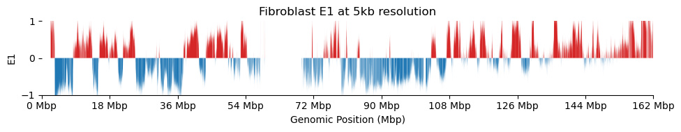
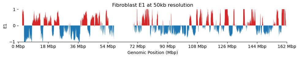
for res in ['1000', '5000', '10000', '50000', '100000']:
    plot_eigenvectors(fib_dict[res], title=f'Fibroblast E1 at {int(int(res)/1000)}kb resolution')
It looks like the 1kb resolution E1 does not reflect A/B-compartmentalization, but only the variance between the three partitions in the viewframe.
I don’t understand that. The partitioning should eliminate the variance between the three partitions, so this could mean that
there is not much variance within the partitions at this resolution
the viewframe is too large
There are a lot of missing values in the 1kb resolution weight and E1, possibly because cooler found that too few contacts were observed to include the bins. That results in a practically unusable E1 track.
# Check how many contacts we have on chrXimport coolerimport globimport osmclrs = glob.glob("../steps/cool/*/*.merged.mcool")clrs = [f"{mcl}::/resolutions/100000"for mcl in mclrs]for clr in clrs: tmp_clr = cooler.Cooler(clr)print(f"""\{os.path.basename(clr.split('::')[0])}:n_chrX contacts: {tmp_clr.pixels().fetch("chrX")['count'].sum():,}\""")
In hindsight, the 1kb resolution Hi-C matrix is way to sparse to do eigendecomposition. From the metadata sheet, there are a total of \(\sim 700,000,000\) Hi-C contacts (\(450,000,000\)cis). Only a fraction of those are on chrX.
Above is the count of total contacts on X on each tissue. It is at most 26,000,000 spread over 160,000 bins at 1kb resolution. That way too sparse to do eigendecomposition.
EEigendecomposition of human sperm sexchromosome separated samples
Here, we prep the E1 values of the data from the human sperm sexchromosome separated samples.
import bioframeimport coolerimport numpy as npimport pandas as pdsperm_X ="../../data/human_sperm_haplo_seperated/sperm_X.merged.mcool"sperm_Y ="../../data/human_sperm_haplo_seperated/sperm_Y.merged.mcool"
# Make viewframesassembly ="GRCh38"centromeres = bioframe.fetch_centromeres(assembly)chromsizes = bioframe.fetch_chromsizes(assembly)chromarms = bioframe.make_chromarms(chromsizes, centromeres)view_x = bioframe.make_viewframe(chromarms).query('chrom == "chrX"')view_y = bioframe.make_viewframe(chromarms).query('chrom == "chrY"')view_x.to_csv(f"../data/view_{assembly}_X_chromarms.tsv", index=False, header=False, sep='\t')view_y.to_csv(f"../data/view_{assembly}_Y_chromarms.tsv", index=False, header=False, sep='\t')# Just for viewspd.concat([view_x, view_y])
chrom
start
end
name
44
chrX
0
61000000
chrX_p
45
chrX
61000000
156040895
chrX_q
46
chrY
0
10400000
chrY_p
47
chrY
10400000
57227415
chrY_q
Calculate the GC contetn coverage
%%bash REF=../../data/human_sperm_haplo_seperated/references/GRCh38.fafor res in100050001000050000100000; do BINS=../data/bins/hg38.bins.${res}.tsv GC_OUT=../data/bins/hg38.gc.${res}.tsv cooltools genome gc $BINS $REF > $GC_OUTdone
Do eigendecomposition
%%bash # Find multires coolersSPERM_X="../../data/human_sperm_haplo_seperated/sperm_X.merged.mcool"SPERM_Y="../../data/human_sperm_haplo_seperated/sperm_Y.merged.mcool"# Define the viewframeVIEW_X=../data/view_GRCh38_X_chromarms.tsvVIEW_Y=../data/view_GRCh38_Y_chromarms.tsv# NamesSAMPLE_X=$(basename $SPERM_X .merged.mcool)SAMPLE_Y=$(basename $SPERM_Y .merged.mcool)echo $SAMPLE_Xfor res in100050001000050000100000500000; do echo $res COOLER=$SPERM_X::resolutions/$res GC_BINS=../data/bins/hg38.gc.${res}.tsv EIGS_OUT=../data/eigs/$SAMPLE_X.eigs.$res echo -ne ' -' $res OK cooltools eigs-cis -o $EIGS_OUT --view $VIEW_X --phasing-track $GC_BINS --n-eigs 3 $COOLERdoneecho ""echo $SAMPLE_Yfor res in100050001000050000100000500000; do echo $res COOLER=$SPERM_Y::resolutions/$res GC_BINS=../data/bins/hg38.gc.${res}.tsv EIGS_OUT=../data/eigs/$SAMPLE_Y.eigs.$res echo -ne ' -' $res OK cooltools eigs-cis -o $EIGS_OUT --view $VIEW_Y --phasing-track $GC_BINS --n-eigs 3 $COOLERdoneecho ""echo All done
sperm_X
1000
/home/sojern/miniconda3/envs/hic/lib/python3.12/site-packages/cooltools/cli/eigs_cis.py:143: FutureWarning: The 'verbose' keyword in pd.read_table is deprecated and will be removed in a future version.
  track_df = pd.read_table(
- 1000 OK5000
/home/sojern/miniconda3/envs/hic/lib/python3.12/site-packages/cooltools/cli/eigs_cis.py:143: FutureWarning: The 'verbose' keyword in pd.read_table is deprecated and will be removed in a future version.
  track_df = pd.read_table(
- 5000 OK10000
/home/sojern/miniconda3/envs/hic/lib/python3.12/site-packages/cooltools/cli/eigs_cis.py:143: FutureWarning: The 'verbose' keyword in pd.read_table is deprecated and will be removed in a future version.
  track_df = pd.read_table(
- 10000 OK50000
/home/sojern/miniconda3/envs/hic/lib/python3.12/site-packages/cooltools/cli/eigs_cis.py:143: FutureWarning: The 'verbose' keyword in pd.read_table is deprecated and will be removed in a future version.
  track_df = pd.read_table(
- 50000 OK100000
/home/sojern/miniconda3/envs/hic/lib/python3.12/site-packages/cooltools/cli/eigs_cis.py:143: FutureWarning: The 'verbose' keyword in pd.read_table is deprecated and will be removed in a future version.
  track_df = pd.read_table(
- 100000 OK500000
/home/sojern/miniconda3/envs/hic/lib/python3.12/site-packages/cooltools/cli/eigs_cis.py:143: FutureWarning: The 'verbose' keyword in pd.read_table is deprecated and will be removed in a future version.
  track_df = pd.read_table(
 - 500000 OK
sperm_Y
1000
/home/sojern/miniconda3/envs/hic/lib/python3.12/site-packages/cooltools/cli/eigs_cis.py:143: FutureWarning: The 'verbose' keyword in pd.read_table is deprecated and will be removed in a future version.
  track_df = pd.read_table(
- 1000 OK5000
/home/sojern/miniconda3/envs/hic/lib/python3.12/site-packages/cooltools/cli/eigs_cis.py:143: FutureWarning: The 'verbose' keyword in pd.read_table is deprecated and will be removed in a future version.
  track_df = pd.read_table(
- 5000 OK10000
/home/sojern/miniconda3/envs/hic/lib/python3.12/site-packages/cooltools/cli/eigs_cis.py:143: FutureWarning: The 'verbose' keyword in pd.read_table is deprecated and will be removed in a future version.
  track_df = pd.read_table(
- 10000 OK50000
/home/sojern/miniconda3/envs/hic/lib/python3.12/site-packages/cooltools/cli/eigs_cis.py:143: FutureWarning: The 'verbose' keyword in pd.read_table is deprecated and will be removed in a future version.
  track_df = pd.read_table(
- 50000 OK100000
/home/sojern/miniconda3/envs/hic/lib/python3.12/site-packages/cooltools/cli/eigs_cis.py:143: FutureWarning: The 'verbose' keyword in pd.read_table is deprecated and will be removed in a future version.
  track_df = pd.read_table(
- 100000 OK500000
/home/sojern/miniconda3/envs/hic/lib/python3.12/site-packages/cooltools/cli/eigs_cis.py:143: FutureWarning: The 'verbose' keyword in pd.read_table is deprecated and will be removed in a future version.
  track_df = pd.read_table(