Comparing GRW models for A/B Clustering

Quantifying differences in GRW models with varying parameters

Here, we compare probabilistic modeling of eigenvectors into A/B compartment calls for Hi-C data.

We compare different models, all using the same underlying structure, but varying smaller aspects of the model.

Goals

To quantify differences in model performance, we use the following metrics:

• WAIC: Widely Applicable Information Criterion, a measure of model fit that penalizes complexity.

• LOO: Leave-One-Out Cross-Validation, a method for estimating the predictive accuracy of a model.

We also try to assign uncertainty to the compartment calls, ultimately defining credible intervals for the compartment transitions.

Imports and setup

import pandas as pd
import numpy as np
import matplotlib.pyplot as plt
import matplotlib_inline
import pymc as pm
import arviz as az
import pytensor.tensor as pt
from scipy.stats import norm, t
from pprint import pprint

## Use a custom style for the plots
plt.style.use('smaller.mplstyle')
matplotlib_inline.backend_inline.set_matplotlib_formats('retina')
#%config InlineBackend.figure_formats = ['retina']

Load/show data

Here, we load the Hi-C contact matrix and the first eigenvector (E1) of the contact matrix. The E1 is used as a predictor for compartment assignment.

The eigendecomposition of the Hi-C matrix was performed with the workflow in the main folder (workflow.py), using the Open2C ecosystem

# Load the data
resolution = 100000

y = pd.Series(pd.read_csv(f"../data/eigs/sperm.eigs.{resolution}.cis.vecs.tsv", sep="\t")['E1'].values.flatten())
x = pd.Series(np.arange(0,y.shape[0])*resolution)

# Make a DataFrame object
df = pd.DataFrame({"start": x, "e1": y})


# Plot the data

fig, ax = plt.subplots(figsize=(10, 3))
ax.fill_between(df.start, df.e1, where=df.e1 > 0, color='tab:red', ec='None', label='E1', step='pre')
ax.fill_between(df.start, df.e1, where=df.e1 < 0, color='tab:blue', ec='None', label='E1', step='pre') 

df.dropna(inplace=True)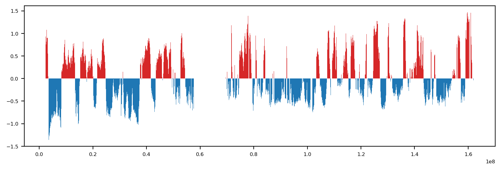

# Histogram of distribution of E1 values (A and B)


x = df["start"].values
y = df["e1"].values
dist_x_values = np.linspace(y.min(), y.max(), 1000)
a_dist = t.pdf(dist_x_values, loc=np.mean(y[y>0]), scale=y[y>0].std(), df=3)
b_dist = t.pdf(dist_x_values, loc=np.mean(y[y<0]), scale=y[y<0].std(), df=3)


f, ax = plt.subplots()

# A compartments
ax.hist(y[y>0], bins=25, color="tab:red", alpha=0.5, label="A", density=True)
# B compartments
ax.hist(y[y<0], bins=25, color="tab:blue", alpha=0.5, label="B", density=True)
# Mean values (vline)
ax.axvline(y[y>0].mean(), color="tab:red", linestyle="--", label="Mean A")
ax.axvline(y[y<0].mean(), color="tab:blue", linestyle="--", label="Mean B")

# Plot the normal distributions
ax.plot(dist_x_values, a_dist, color="tab:red", label="Stud A")
ax.plot(dist_x_values, b_dist, color="tab:blue", label="Stud B")
ax.plot(dist_x_values, a_dist+b_dist, color="tab:purple", label="Stacked StudT")

# Final touches
plt.xlabel("E1")
plt.ylabel("Density")
plt.legend(loc='best')
plt.tight_layout()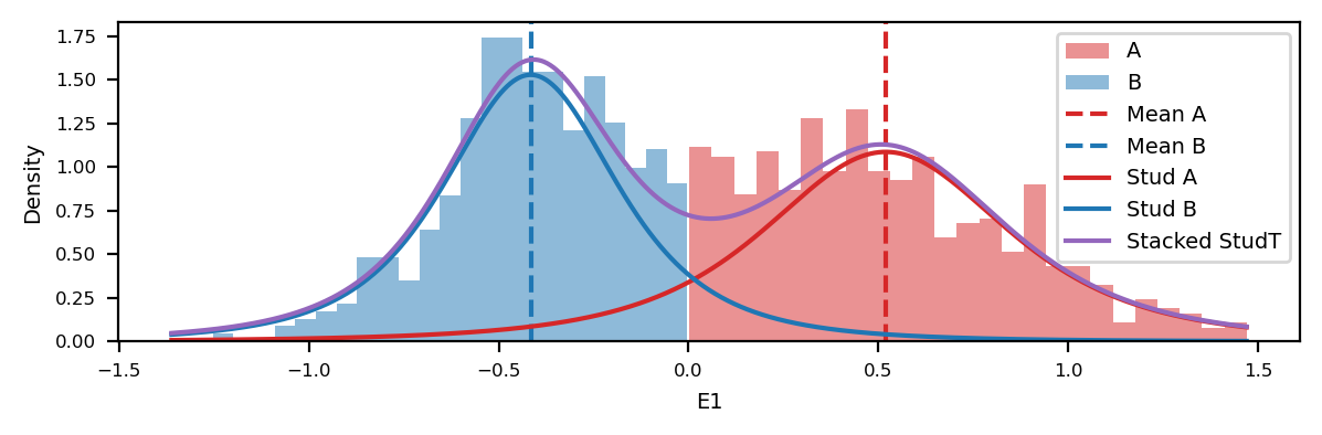

Here, the observed distributions are compared to StudenT distributions of 3 degrees of freedom and the same mean and standard deviation as the observed data. The Student’s t-distribution is used because it is more robust with its heavier tails than the normal.

Models

Here, we expand on the results from 03_PyMC_GRW_logit.ipynb, and use the same model structure, but with different priors and likelihoods. Overall, the following thoughts are implemented:

• We assume that the eigenvectors can be drawn from a mixture of two distributions, one for each compartment (A and B). It could be any mixture, but the means should be negative for B and positive for A. We use either to model mu:
  • Gaussians, as a simple starting point, or
  • Student’s t-distributions, as a heavier-tailed alternative.
  • The mixtures has to be ordered in PyMC to ensure that the A compartment is always positive and the B compartment is always negative.
• The mixture components have their own (learned) standard deviation, sigma.
• The mixture components use mu and sigma (each of shape 2) in either a,
  • Normal distribution, or
  • Student’s t-distribution, with 10 degrees of freedom.
• We model the mixture weight as a non-centered (Gaussian) random walk prior, as a method of probabilistic smoothing of the PCA compartment calls.
  • eps is the (learned) step size of the random walk, and
    • either Normal or Student’s t-distributed
  • grw_sigma is the (learned) standard deviation of the random walk
    • either HalfNormal or HalfStudentT-distributed
  • The logit-space (of the mixture weight) is then modeled deterministically as the cummulative sum of the random walk steps.
  • The logit-space is then transformed to the probability space by squishing it through a sigmoid function.
• \(\hat{y}\) (y_hat) is drawing the observations from the mixture distribution, using the mixture weight and the two components (the learned distributions of E1 values for A and B-compartments).

Model 1: T-dist in logit space, T-dist in mixture components

import pytensor.tensor as pt

with pm.Model(coords={"pos": df.index.values}) as latentT_Tmix_model:
    e1 = pm.Data("e1", df.e1.values, dims="pos")

    # Ordered parameters for the means of the two components
    # Note: The ordered transform ensures that mu_a < mu_b
    mu = pm.Normal("mu", mu=[-0.5, 0.5], sigma=0.3,
        transform=pm.distributions.transforms.ordered, # IMPORTANT
        shape=2,
        )
    sigma = pm.HalfNormal("sigma", 0.3, shape=2)

    # GRW over logit space; non-centered reparameterization
    grw_sigma = pm.HalfNormal("grw_sigma", 0.05)

    # StudentT distribution for eps (got alot of divergences with nu=3)
    eps = pm.StudentT("eps", nu=10, mu=0.0, sigma=1.0, dims="pos")
    
    # Cumulative sum to create a Gaussian Random Walk
    logit_w = pm.Deterministic("logit_w", pt.cumsum(eps * grw_sigma), dims="pos")
    w = pm.Deterministic("w", pm.math.sigmoid(logit_w), dims="pos")

    # Components of the mixture model
    components = pm.StudentT.dist(nu=10, mu=mu, sigma=sigma, shape=2)

    # Mixture model
    # The observed data is modeled as a mixture of the two components
    y_hat = pm.Mixture("y_hat", w=pm.math.stack([w,1-w], axis=1), comp_dists=components, observed=e1, dims='pos')

Model 1: T-dist in logit space, Normal in mixture components

with pm.Model(coords={"pos": df.index.values}) as latentT_Nmix_model:
    e1 = pm.Data("e1", df.e1.values, dims="pos")

    # Ordered parameters for the means of the two components
    # Note: The ordered transform ensures that mu_a < mu_b
    mu = pm.Normal("mu", mu=[-0.5, 0.5], sigma=0.3,
        transform=pm.distributions.transforms.ordered, # IMPORTANT
        shape=2,
        )
    sigma = pm.HalfNormal("sigma", 0.3, shape=2)

    # GRW over logit space; non-centered reparameterization
    grw_sigma = pm.HalfNormal("grw_sigma", 0.05)

    # StudentT distribution for eps (got alot of divergences with nu=3)
    eps = pm.StudentT("eps", nu=10, mu=0.0, sigma=1.0, dims="pos")
    
    # Cumulative sum to create a Gaussian Random Walk
    logit_w = pm.Deterministic("logit_w", pt.cumsum(eps * grw_sigma), dims="pos")
    w = pm.Deterministic("w", pm.math.sigmoid(logit_w), dims="pos")

    # Components of the mixture model
    components = pm.StudentT.dist(nu=10, mu=mu, sigma=sigma, shape=2)

    # Mixture model
    # The observed data is modeled as a mixture of the two components
    y_hat = pm.Mixture("y_hat", w=pm.math.stack([w,1-w], axis=1), comp_dists=components, observed=e1, dims='pos')

Parameter sweep configuration

Here is an attempt to sweep through parameters in a reproducible and deterministic way. The idea is to use a grid search over the parameters, and then run the models in parallel, and finally collect the results and analyze them.

First, let’s create a function that create a grid of parameters to sweep over using itertools.

Create parameter grid

import itertools as it

def create_model_grid():
    """
    Create a grid of models for the different configurations as defined below.
    Name the model according to the configuration for easier identification:
    - comp_dist: Distribution of the components (Normal or StudentT)
    - eps_dist: Distribution of the GRW steps (Normal or StudentT)
    - grw_sigma_dist: Distribution of the GRW noise (HalfNormal or HalfStudentT)
    name = f"{comp_dist}_{eps_dist}_{grw_sigma_dist}"
    - If any distribution is StudentT, append the nu parameter to the name.
    """

    def config_namer(comp_dist, comp_kwargs, eps_dist, eps_kwargs, grw_sigma_dist, grw_sigma_kwargs):
        abbr = {
            'Normal': 'N',
            'StudentT': 'T',
            'HalfNormal': 'HN',
            'HalfStudentT': 'HT'
        }

        name = f"{abbr[comp_dist]}_{abbr[eps_dist]}_{abbr[grw_sigma_dist]}"
        if comp_dist == 'StudentT':
            name += f"_{comp_kwargs['nu']}"
        if eps_dist == 'StudentT':
            name += f"_{eps_kwargs['nu']}"
        if grw_sigma_dist == 'HalfStudentT':
            name += f"_{grw_sigma_kwargs['nu']}"
        return name
    
    comp_kwargs_list = [
    ('Normal', {}),
    ('StudentT', {'nu': 10}),
    ('StudentT', {'nu': 5})
    ]

    eps_kwargs_list = [
        ('Normal', {'mu': 0.0, 'sigma': 1.0}),
        ('StudentT', {'nu': 10, 'mu': 0.0, 'sigma': 1.0}),
        ('StudentT', {'nu': 5, 'mu': 0.0, 'sigma': 0.5})
    ]

    grw_sigma_kwargs_list = [
        ('HalfNormal', {'sigma': 0.05}),
        ('HalfStudentT', {'nu': 10, 'sigma': 0.05}),
        ('HalfStudentT', {'nu': 5, 'sigma': 0.01})
    ]


    # Prior configurations for E1 mixture
    mu_mu = [-0.5, 0.5]
    mu_sigma = 0.3
    sigma = 0.3

    grid = it.product(comp_kwargs_list, eps_kwargs_list, grw_sigma_kwargs_list)
    configs = []
    for (comp_dist, comp_kwargs), (eps_dist, eps_kwargs), (grw_sigma_dist, grw_sigma_kwargs) in grid:
        name = config_namer(
            comp_dist, comp_kwargs, 
            eps_dist, eps_kwargs, 
            grw_sigma_dist, grw_sigma_kwargs
            )
        config = {
            'name': name,
            'comp_dist': comp_dist,
            'comp_kwargs': comp_kwargs,
            'eps_dist': eps_dist,
            'eps_kwargs': eps_kwargs,
            'grw_sigma_dist': grw_sigma_dist,
            'grw_sigma_kwargs': grw_sigma_kwargs,
            'mu_mu': mu_mu,
            'mu_sigma': mu_sigma,
            'sigma': sigma
        }
        configs.append(config)
    return configs

from pprint import pprint
import json
# Instantiate the model grid
configs = create_model_grid()

pprint(configs)

# Save the model grid to a JSON file
with open("../results/model_grid.json", "w") as f:
    json.dump(configs, f, indent=4)

[{'comp_dist': 'Normal',
  'comp_kwargs': {},
  'eps_dist': 'Normal',
  'eps_kwargs': {'mu': 0.0, 'sigma': 1.0},
  'grw_sigma_dist': 'HalfNormal',
  'grw_sigma_kwargs': {'sigma': 0.05},
  'mu_mu': [-0.5, 0.5],
  'mu_sigma': 0.3,
  'name': 'N_N_HN',
  'sigma': 0.3},
 {'comp_dist': 'Normal',
  'comp_kwargs': {},
  'eps_dist': 'Normal',
  'eps_kwargs': {'mu': 0.0, 'sigma': 1.0},
  'grw_sigma_dist': 'HalfStudentT',
  'grw_sigma_kwargs': {'nu': 10, 'sigma': 0.05},
  'mu_mu': [-0.5, 0.5],
  'mu_sigma': 0.3,
  'name': 'N_N_HT_10',
  'sigma': 0.3},
 {'comp_dist': 'Normal',
  'comp_kwargs': {},
  'eps_dist': 'Normal',
  'eps_kwargs': {'mu': 0.0, 'sigma': 1.0},
  'grw_sigma_dist': 'HalfStudentT',
  'grw_sigma_kwargs': {'nu': 5, 'sigma': 0.01},
  'mu_mu': [-0.5, 0.5],
  'mu_sigma': 0.3,
  'name': 'N_N_HT_5',
  'sigma': 0.3},
 {'comp_dist': 'Normal',
  'comp_kwargs': {},
  'eps_dist': 'StudentT',
  'eps_kwargs': {'mu': 0.0, 'nu': 10, 'sigma': 1.0},
  'grw_sigma_dist': 'HalfNormal',
  'grw_sigma_kwargs': {'sigma': 0.05},
  'mu_mu': [-0.5, 0.5],
  'mu_sigma': 0.3,
  'name': 'N_T_HN_10',
  'sigma': 0.3},
 {'comp_dist': 'Normal',
  'comp_kwargs': {},
  'eps_dist': 'StudentT',
  'eps_kwargs': {'mu': 0.0, 'nu': 10, 'sigma': 1.0},
  'grw_sigma_dist': 'HalfStudentT',
  'grw_sigma_kwargs': {'nu': 10, 'sigma': 0.05},
  'mu_mu': [-0.5, 0.5],
  'mu_sigma': 0.3,
  'name': 'N_T_HT_10_10',
  'sigma': 0.3},
 {'comp_dist': 'Normal',
  'comp_kwargs': {},
  'eps_dist': 'StudentT',
  'eps_kwargs': {'mu': 0.0, 'nu': 10, 'sigma': 1.0},
  'grw_sigma_dist': 'HalfStudentT',
  'grw_sigma_kwargs': {'nu': 5, 'sigma': 0.01},
  'mu_mu': [-0.5, 0.5],
  'mu_sigma': 0.3,
  'name': 'N_T_HT_10_5',
  'sigma': 0.3},
 {'comp_dist': 'Normal',
  'comp_kwargs': {},
  'eps_dist': 'StudentT',
  'eps_kwargs': {'mu': 0.0, 'nu': 5, 'sigma': 0.5},
  'grw_sigma_dist': 'HalfNormal',
  'grw_sigma_kwargs': {'sigma': 0.05},
  'mu_mu': [-0.5, 0.5],
  'mu_sigma': 0.3,
  'name': 'N_T_HN_5',
  'sigma': 0.3},
 {'comp_dist': 'Normal',
  'comp_kwargs': {},
  'eps_dist': 'StudentT',
  'eps_kwargs': {'mu': 0.0, 'nu': 5, 'sigma': 0.5},
  'grw_sigma_dist': 'HalfStudentT',
  'grw_sigma_kwargs': {'nu': 10, 'sigma': 0.05},
  'mu_mu': [-0.5, 0.5],
  'mu_sigma': 0.3,
  'name': 'N_T_HT_5_10',
  'sigma': 0.3},
 {'comp_dist': 'Normal',
  'comp_kwargs': {},
  'eps_dist': 'StudentT',
  'eps_kwargs': {'mu': 0.0, 'nu': 5, 'sigma': 0.5},
  'grw_sigma_dist': 'HalfStudentT',
  'grw_sigma_kwargs': {'nu': 5, 'sigma': 0.01},
  'mu_mu': [-0.5, 0.5],
  'mu_sigma': 0.3,
  'name': 'N_T_HT_5_5',
  'sigma': 0.3},
 {'comp_dist': 'StudentT',
  'comp_kwargs': {'nu': 10},
  'eps_dist': 'Normal',
  'eps_kwargs': {'mu': 0.0, 'sigma': 1.0},
  'grw_sigma_dist': 'HalfNormal',
  'grw_sigma_kwargs': {'sigma': 0.05},
  'mu_mu': [-0.5, 0.5],
  'mu_sigma': 0.3,
  'name': 'T_N_HN_10',
  'sigma': 0.3},
 {'comp_dist': 'StudentT',
  'comp_kwargs': {'nu': 10},
  'eps_dist': 'Normal',
  'eps_kwargs': {'mu': 0.0, 'sigma': 1.0},
  'grw_sigma_dist': 'HalfStudentT',
  'grw_sigma_kwargs': {'nu': 10, 'sigma': 0.05},
  'mu_mu': [-0.5, 0.5],
  'mu_sigma': 0.3,
  'name': 'T_N_HT_10_10',
  'sigma': 0.3},
 {'comp_dist': 'StudentT',
  'comp_kwargs': {'nu': 10},
  'eps_dist': 'Normal',
  'eps_kwargs': {'mu': 0.0, 'sigma': 1.0},
  'grw_sigma_dist': 'HalfStudentT',
  'grw_sigma_kwargs': {'nu': 5, 'sigma': 0.01},
  'mu_mu': [-0.5, 0.5],
  'mu_sigma': 0.3,
  'name': 'T_N_HT_10_5',
  'sigma': 0.3},
 {'comp_dist': 'StudentT',
  'comp_kwargs': {'nu': 10},
  'eps_dist': 'StudentT',
  'eps_kwargs': {'mu': 0.0, 'nu': 10, 'sigma': 1.0},
  'grw_sigma_dist': 'HalfNormal',
  'grw_sigma_kwargs': {'sigma': 0.05},
  'mu_mu': [-0.5, 0.5],
  'mu_sigma': 0.3,
  'name': 'T_T_HN_10_10',
  'sigma': 0.3},
 {'comp_dist': 'StudentT',
  'comp_kwargs': {'nu': 10},
  'eps_dist': 'StudentT',
  'eps_kwargs': {'mu': 0.0, 'nu': 10, 'sigma': 1.0},
  'grw_sigma_dist': 'HalfStudentT',
  'grw_sigma_kwargs': {'nu': 10, 'sigma': 0.05},
  'mu_mu': [-0.5, 0.5],
  'mu_sigma': 0.3,
  'name': 'T_T_HT_10_10_10',
  'sigma': 0.3},
 {'comp_dist': 'StudentT',
  'comp_kwargs': {'nu': 10},
  'eps_dist': 'StudentT',
  'eps_kwargs': {'mu': 0.0, 'nu': 10, 'sigma': 1.0},
  'grw_sigma_dist': 'HalfStudentT',
  'grw_sigma_kwargs': {'nu': 5, 'sigma': 0.01},
  'mu_mu': [-0.5, 0.5],
  'mu_sigma': 0.3,
  'name': 'T_T_HT_10_10_5',
  'sigma': 0.3},
 {'comp_dist': 'StudentT',
  'comp_kwargs': {'nu': 10},
  'eps_dist': 'StudentT',
  'eps_kwargs': {'mu': 0.0, 'nu': 5, 'sigma': 0.5},
  'grw_sigma_dist': 'HalfNormal',
  'grw_sigma_kwargs': {'sigma': 0.05},
  'mu_mu': [-0.5, 0.5],
  'mu_sigma': 0.3,
  'name': 'T_T_HN_10_5',
  'sigma': 0.3},
 {'comp_dist': 'StudentT',
  'comp_kwargs': {'nu': 10},
  'eps_dist': 'StudentT',
  'eps_kwargs': {'mu': 0.0, 'nu': 5, 'sigma': 0.5},
  'grw_sigma_dist': 'HalfStudentT',
  'grw_sigma_kwargs': {'nu': 10, 'sigma': 0.05},
  'mu_mu': [-0.5, 0.5],
  'mu_sigma': 0.3,
  'name': 'T_T_HT_10_5_10',
  'sigma': 0.3},
 {'comp_dist': 'StudentT',
  'comp_kwargs': {'nu': 10},
  'eps_dist': 'StudentT',
  'eps_kwargs': {'mu': 0.0, 'nu': 5, 'sigma': 0.5},
  'grw_sigma_dist': 'HalfStudentT',
  'grw_sigma_kwargs': {'nu': 5, 'sigma': 0.01},
  'mu_mu': [-0.5, 0.5],
  'mu_sigma': 0.3,
  'name': 'T_T_HT_10_5_5',
  'sigma': 0.3},
 {'comp_dist': 'StudentT',
  'comp_kwargs': {'nu': 5},
  'eps_dist': 'Normal',
  'eps_kwargs': {'mu': 0.0, 'sigma': 1.0},
  'grw_sigma_dist': 'HalfNormal',
  'grw_sigma_kwargs': {'sigma': 0.05},
  'mu_mu': [-0.5, 0.5],
  'mu_sigma': 0.3,
  'name': 'T_N_HN_5',
  'sigma': 0.3},
 {'comp_dist': 'StudentT',
  'comp_kwargs': {'nu': 5},
  'eps_dist': 'Normal',
  'eps_kwargs': {'mu': 0.0, 'sigma': 1.0},
  'grw_sigma_dist': 'HalfStudentT',
  'grw_sigma_kwargs': {'nu': 10, 'sigma': 0.05},
  'mu_mu': [-0.5, 0.5],
  'mu_sigma': 0.3,
  'name': 'T_N_HT_5_10',
  'sigma': 0.3},
 {'comp_dist': 'StudentT',
  'comp_kwargs': {'nu': 5},
  'eps_dist': 'Normal',
  'eps_kwargs': {'mu': 0.0, 'sigma': 1.0},
  'grw_sigma_dist': 'HalfStudentT',
  'grw_sigma_kwargs': {'nu': 5, 'sigma': 0.01},
  'mu_mu': [-0.5, 0.5],
  'mu_sigma': 0.3,
  'name': 'T_N_HT_5_5',
  'sigma': 0.3},
 {'comp_dist': 'StudentT',
  'comp_kwargs': {'nu': 5},
  'eps_dist': 'StudentT',
  'eps_kwargs': {'mu': 0.0, 'nu': 10, 'sigma': 1.0},
  'grw_sigma_dist': 'HalfNormal',
  'grw_sigma_kwargs': {'sigma': 0.05},
  'mu_mu': [-0.5, 0.5],
  'mu_sigma': 0.3,
  'name': 'T_T_HN_5_10',
  'sigma': 0.3},
 {'comp_dist': 'StudentT',
  'comp_kwargs': {'nu': 5},
  'eps_dist': 'StudentT',
  'eps_kwargs': {'mu': 0.0, 'nu': 10, 'sigma': 1.0},
  'grw_sigma_dist': 'HalfStudentT',
  'grw_sigma_kwargs': {'nu': 10, 'sigma': 0.05},
  'mu_mu': [-0.5, 0.5],
  'mu_sigma': 0.3,
  'name': 'T_T_HT_5_10_10',
  'sigma': 0.3},
 {'comp_dist': 'StudentT',
  'comp_kwargs': {'nu': 5},
  'eps_dist': 'StudentT',
  'eps_kwargs': {'mu': 0.0, 'nu': 10, 'sigma': 1.0},
  'grw_sigma_dist': 'HalfStudentT',
  'grw_sigma_kwargs': {'nu': 5, 'sigma': 0.01},
  'mu_mu': [-0.5, 0.5],
  'mu_sigma': 0.3,
  'name': 'T_T_HT_5_10_5',
  'sigma': 0.3},
 {'comp_dist': 'StudentT',
  'comp_kwargs': {'nu': 5},
  'eps_dist': 'StudentT',
  'eps_kwargs': {'mu': 0.0, 'nu': 5, 'sigma': 0.5},
  'grw_sigma_dist': 'HalfNormal',
  'grw_sigma_kwargs': {'sigma': 0.05},
  'mu_mu': [-0.5, 0.5],
  'mu_sigma': 0.3,
  'name': 'T_T_HN_5_5',
  'sigma': 0.3},
 {'comp_dist': 'StudentT',
  'comp_kwargs': {'nu': 5},
  'eps_dist': 'StudentT',
  'eps_kwargs': {'mu': 0.0, 'nu': 5, 'sigma': 0.5},
  'grw_sigma_dist': 'HalfStudentT',
  'grw_sigma_kwargs': {'nu': 10, 'sigma': 0.05},
  'mu_mu': [-0.5, 0.5],
  'mu_sigma': 0.3,
  'name': 'T_T_HT_5_5_10',
  'sigma': 0.3},
 {'comp_dist': 'StudentT',
  'comp_kwargs': {'nu': 5},
  'eps_dist': 'StudentT',
  'eps_kwargs': {'mu': 0.0, 'nu': 5, 'sigma': 0.5},
  'grw_sigma_dist': 'HalfStudentT',
  'grw_sigma_kwargs': {'nu': 5, 'sigma': 0.01},
  'mu_mu': [-0.5, 0.5],
  'mu_sigma': 0.3,
  'name': 'T_T_HT_5_5_5',
  'sigma': 0.3}]

Create model builder function

Then, we want to create a function (model_builder) that takes the parameters and returns a PyMC model. This function will be used to build the models in parallel.

NOTE: accidentally, I switched the order of mixture weights, so the posterior mean of w now determines the probability of being in a B compartment (coming from the distribution with negative mean)

def build_model_from_config(df, cfg):
    """
    Build a PyMC model based on the provided configuration dictionary.
    """

    with pm.Model(coords={"pos": df.index.values}) as model:
        e1 = pm.Data("e1", df.e1.values, dims="pos")

        mu = pm.Normal("mu", mu=cfg['mu_mu'], sigma=cfg['mu_sigma'],
                       transform=pm.distributions.transforms.ordered, shape=2)
        sigma = pm.HalfNormal("sigma", sigma=cfg['sigma'], shape=2)

        # components: Normal or StudentT
        if cfg['comp_dist'] == "Normal":
            components = pm.Normal.dist(mu=mu, sigma=sigma, shape=2)
        else:
            components = pm.StudentT.dist(mu=mu, sigma=sigma, **cfg['comp_kwargs'], shape=2)

        # grw_sigma: HalfNormal or HalfStudentT
        if cfg['grw_sigma_dist'] == "HalfNormal":
            grw_sigma = pm.HalfNormal("grw_sigma", **cfg['grw_sigma_kwargs'])
        else:
            grw_sigma = pm.HalfStudentT("grw_sigma", **cfg['grw_sigma_kwargs'])

        # eps: Normal or StudentT
        if cfg['eps_dist'] == "Normal":
            eps = pm.Normal("eps", dims="pos", **cfg['eps_kwargs'])
        else:
            eps = pm.StudentT("eps", dims="pos", **cfg['eps_kwargs'])

        logit_w = pm.Deterministic("logit_w", pt.cumsum(eps * grw_sigma), dims="pos")
        w = pm.Deterministic("w", pm.math.sigmoid(logit_w), dims="pos")

        y_hat = pm.Mixture("y_hat", w=pt.stack([w, 1-w], axis=1), comp_dists=components,
                           observed=e1, dims='pos')

    return model

Sampling loop

Now, we create the sampling loop that should run the models in sequence.

We will name the models by joining the list [number, comp_dist, eps_dist, grw_sigma_dist][eps_nu, comp_nu].

All the traces (InferenceData) will be saved in a dictionary, model_traces.

Sample the models

from datetime import datetime

def log(msg, path=".04_PyMC_GRW_compare.log", overwrite=False):
    print(f"LOG: {msg}")
    if overwrite:
        with open(path, "w") as f:
            f.write(msg + "\n")
    else:
        with open(path, "a") as f:
            f.write(msg + "\n")


# Reset the log file
log("Resetting log... \n", overwrite=True)

model_traces = {}

for i, cfg in enumerate(configs):
    name = cfg['name']
    
    if name in model_traces:
        continue
    else:
        model_traces[name] = {'model': None, 'trace': None, 'scores': None}


    log(f"Sampling {name}...")
    try:
        start = datetime.now()
        log(f"Started at {start.strftime('%H:%M:%S')}")
        model_traces[name]['model'] = build_model_from_config(df, cfg)
        model = model_traces[name]['model']
        trace = pm.sample(draws=1000, tune=1000, chains=7, cores=7, progressbar=False, model=model)
        model_traces[name]['trace'] = trace
        log(f"--> Took {(datetime.now()-start).total_seconds()} seconds!\n")
    except Exception as e:
        log(f"Model {name} failed: {e}\n")

LOG: Resetting log... 

LOG: Sampling N_N_HN...
LOG: Started at 22:36:58

Initializing NUTS using jitter+adapt_diag...
Multiprocess sampling (7 chains in 7 jobs)
NUTS: [mu, sigma, grw_sigma, eps]
Sampling 7 chains for 1_000 tune and 1_000 draw iterations (7_000 + 7_000 draws total) took 302 seconds.

LOG: --> Took 310.351568 seconds!

LOG: Sampling N_N_HT_10...
LOG: Started at 22:42:09

Initializing NUTS using jitter+adapt_diag...
Multiprocess sampling (7 chains in 7 jobs)
NUTS: [mu, sigma, grw_sigma, eps]
Sampling 7 chains for 1_000 tune and 1_000 draw iterations (7_000 + 7_000 draws total) took 107 seconds.
There were 6980 divergences after tuning. Increase `target_accept` or reparameterize.
The rhat statistic is larger than 1.01 for some parameters. This indicates problems during sampling. See https://arxiv.org/abs/1903.08008 for details
The effective sample size per chain is smaller than 100 for some parameters.  A higher number is needed for reliable rhat and ess computation. See https://arxiv.org/abs/1903.08008 for details

LOG: --> Took 118.167902 seconds!

LOG: Sampling N_N_HT_5...
LOG: Started at 22:44:07

Initializing NUTS using jitter+adapt_diag...
Multiprocess sampling (7 chains in 7 jobs)
NUTS: [mu, sigma, grw_sigma, eps]
Sampling 7 chains for 1_000 tune and 1_000 draw iterations (7_000 + 7_000 draws total) took 134 seconds.
There were 6851 divergences after tuning. Increase `target_accept` or reparameterize.
Chain 6 reached the maximum tree depth. Increase `max_treedepth`, increase `target_accept` or reparameterize.
The rhat statistic is larger than 1.01 for some parameters. This indicates problems during sampling. See https://arxiv.org/abs/1903.08008 for details
The effective sample size per chain is smaller than 100 for some parameters.  A higher number is needed for reliable rhat and ess computation. See https://arxiv.org/abs/1903.08008 for details

LOG: --> Took 143.521094 seconds!

LOG: Sampling N_T_HN_10...
LOG: Started at 22:46:30

Initializing NUTS using jitter+adapt_diag...
Multiprocess sampling (7 chains in 7 jobs)
NUTS: [mu, sigma, grw_sigma, eps]
Sampling 7 chains for 1_000 tune and 1_000 draw iterations (7_000 + 7_000 draws total) took 320 seconds.

LOG: --> Took 326.008741 seconds!

LOG: Sampling N_T_HT_10_10...
LOG: Started at 22:51:56

Initializing NUTS using jitter+adapt_diag...
Multiprocess sampling (7 chains in 7 jobs)
NUTS: [mu, sigma, grw_sigma, eps]
Sampling 7 chains for 1_000 tune and 1_000 draw iterations (7_000 + 7_000 draws total) took 157 seconds.
There were 6843 divergences after tuning. Increase `target_accept` or reparameterize.
Chain 6 reached the maximum tree depth. Increase `max_treedepth`, increase `target_accept` or reparameterize.
The rhat statistic is larger than 1.01 for some parameters. This indicates problems during sampling. See https://arxiv.org/abs/1903.08008 for details
The effective sample size per chain is smaller than 100 for some parameters.  A higher number is needed for reliable rhat and ess computation. See https://arxiv.org/abs/1903.08008 for details

LOG: --> Took 166.726683 seconds!

LOG: Sampling N_T_HT_10_5...
LOG: Started at 22:54:43

Initializing NUTS using jitter+adapt_diag...
Multiprocess sampling (7 chains in 7 jobs)
NUTS: [mu, sigma, grw_sigma, eps]
Sampling 7 chains for 1_000 tune and 1_000 draw iterations (7_000 + 7_000 draws total) took 76 seconds.
There were 6997 divergences after tuning. Increase `target_accept` or reparameterize.
The rhat statistic is larger than 1.01 for some parameters. This indicates problems during sampling. See https://arxiv.org/abs/1903.08008 for details
The effective sample size per chain is smaller than 100 for some parameters.  A higher number is needed for reliable rhat and ess computation. See https://arxiv.org/abs/1903.08008 for details

LOG: --> Took 85.394018 seconds!

LOG: Sampling N_T_HN_5...
LOG: Started at 22:56:08

Initializing NUTS using jitter+adapt_diag...
Multiprocess sampling (7 chains in 7 jobs)
NUTS: [mu, sigma, grw_sigma, eps]
Sampling 7 chains for 1_000 tune and 1_000 draw iterations (7_000 + 7_000 draws total) took 229 seconds.
The rhat statistic is larger than 1.01 for some parameters. This indicates problems during sampling. See https://arxiv.org/abs/1903.08008 for details
The effective sample size per chain is smaller than 100 for some parameters.  A higher number is needed for reliable rhat and ess computation. See https://arxiv.org/abs/1903.08008 for details

LOG: --> Took 240.948306 seconds!

LOG: Sampling N_T_HT_5_10...
LOG: Started at 23:00:09

Initializing NUTS using jitter+adapt_diag...
Multiprocess sampling (7 chains in 7 jobs)
NUTS: [mu, sigma, grw_sigma, eps]
Sampling 7 chains for 1_000 tune and 1_000 draw iterations (7_000 + 7_000 draws total) took 164 seconds.
There were 6873 divergences after tuning. Increase `target_accept` or reparameterize.
Chain 4 reached the maximum tree depth. Increase `max_treedepth`, increase `target_accept` or reparameterize.
The rhat statistic is larger than 1.01 for some parameters. This indicates problems during sampling. See https://arxiv.org/abs/1903.08008 for details
The effective sample size per chain is smaller than 100 for some parameters.  A higher number is needed for reliable rhat and ess computation. See https://arxiv.org/abs/1903.08008 for details

LOG: --> Took 174.36611 seconds!

LOG: Sampling N_T_HT_5_5...
LOG: Started at 23:03:04

Initializing NUTS using jitter+adapt_diag...
Multiprocess sampling (7 chains in 7 jobs)
NUTS: [mu, sigma, grw_sigma, eps]
Sampling 7 chains for 1_000 tune and 1_000 draw iterations (7_000 + 7_000 draws total) took 91 seconds.
There were 6999 divergences after tuning. Increase `target_accept` or reparameterize.
The rhat statistic is larger than 1.01 for some parameters. This indicates problems during sampling. See https://arxiv.org/abs/1903.08008 for details
The effective sample size per chain is smaller than 100 for some parameters.  A higher number is needed for reliable rhat and ess computation. See https://arxiv.org/abs/1903.08008 for details

LOG: --> Took 101.124336 seconds!

LOG: Sampling T_N_HN_10...
LOG: Started at 23:04:45

Initializing NUTS using jitter+adapt_diag...
Multiprocess sampling (7 chains in 7 jobs)
NUTS: [mu, sigma, grw_sigma, eps]
Sampling 7 chains for 1_000 tune and 1_000 draw iterations (7_000 + 7_000 draws total) took 359 seconds.

LOG: --> Took 365.130255 seconds!

LOG: Sampling T_N_HT_10_10...
LOG: Started at 23:10:50

Initializing NUTS using jitter+adapt_diag...
Multiprocess sampling (7 chains in 7 jobs)
NUTS: [mu, sigma, grw_sigma, eps]
Sampling 7 chains for 1_000 tune and 1_000 draw iterations (7_000 + 7_000 draws total) took 122 seconds.
There were 6989 divergences after tuning. Increase `target_accept` or reparameterize.
The rhat statistic is larger than 1.01 for some parameters. This indicates problems during sampling. See https://arxiv.org/abs/1903.08008 for details
The effective sample size per chain is smaller than 100 for some parameters.  A higher number is needed for reliable rhat and ess computation. See https://arxiv.org/abs/1903.08008 for details

LOG: --> Took 132.235343 seconds!

LOG: Sampling T_N_HT_10_5...
LOG: Started at 23:13:02

Initializing NUTS using jitter+adapt_diag...
Multiprocess sampling (7 chains in 7 jobs)
NUTS: [mu, sigma, grw_sigma, eps]
Sampling 7 chains for 1_000 tune and 1_000 draw iterations (7_000 + 7_000 draws total) took 171 seconds.
There were 6805 divergences after tuning. Increase `target_accept` or reparameterize.
Chain 0 reached the maximum tree depth. Increase `max_treedepth`, increase `target_accept` or reparameterize.
The rhat statistic is larger than 1.01 for some parameters. This indicates problems during sampling. See https://arxiv.org/abs/1903.08008 for details
The effective sample size per chain is smaller than 100 for some parameters.  A higher number is needed for reliable rhat and ess computation. See https://arxiv.org/abs/1903.08008 for details

LOG: --> Took 181.227185 seconds!

LOG: Sampling T_T_HN_10_10...
LOG: Started at 23:16:03

Initializing NUTS using jitter+adapt_diag...
Multiprocess sampling (7 chains in 7 jobs)
NUTS: [mu, sigma, grw_sigma, eps]
Sampling 7 chains for 1_000 tune and 1_000 draw iterations (7_000 + 7_000 draws total) took 366 seconds.

LOG: --> Took 372.410547 seconds!

LOG: Sampling T_T_HT_10_10_10...
LOG: Started at 23:22:16

Initializing NUTS using jitter+adapt_diag...
Multiprocess sampling (7 chains in 7 jobs)
NUTS: [mu, sigma, grw_sigma, eps]
Sampling 7 chains for 1_000 tune and 1_000 draw iterations (7_000 + 7_000 draws total) took 103 seconds.
There were 6999 divergences after tuning. Increase `target_accept` or reparameterize.
The rhat statistic is larger than 1.01 for some parameters. This indicates problems during sampling. See https://arxiv.org/abs/1903.08008 for details
The effective sample size per chain is smaller than 100 for some parameters.  A higher number is needed for reliable rhat and ess computation. See https://arxiv.org/abs/1903.08008 for details

LOG: --> Took 113.559086 seconds!

LOG: Sampling T_T_HT_10_10_5...
LOG: Started at 23:24:09

Initializing NUTS using jitter+adapt_diag...
Multiprocess sampling (7 chains in 7 jobs)
NUTS: [mu, sigma, grw_sigma, eps]
Sampling 7 chains for 1_000 tune and 1_000 draw iterations (7_000 + 7_000 draws total) took 164 seconds.
There were 6969 divergences after tuning. Increase `target_accept` or reparameterize.
The rhat statistic is larger than 1.01 for some parameters. This indicates problems during sampling. See https://arxiv.org/abs/1903.08008 for details
The effective sample size per chain is smaller than 100 for some parameters.  A higher number is needed for reliable rhat and ess computation. See https://arxiv.org/abs/1903.08008 for details

LOG: --> Took 173.920995 seconds!

LOG: Sampling T_T_HN_10_5...
LOG: Started at 23:27:03

Initializing NUTS using jitter+adapt_diag...
Multiprocess sampling (7 chains in 7 jobs)
NUTS: [mu, sigma, grw_sigma, eps]
Sampling 7 chains for 1_000 tune and 1_000 draw iterations (7_000 + 7_000 draws total) took 241 seconds.
The rhat statistic is larger than 1.01 for some parameters. This indicates problems during sampling. See https://arxiv.org/abs/1903.08008 for details

LOG: --> Took 246.952836 seconds!

LOG: Sampling T_T_HT_10_5_10...
LOG: Started at 23:31:10

Initializing NUTS using jitter+adapt_diag...
Multiprocess sampling (7 chains in 7 jobs)
NUTS: [mu, sigma, grw_sigma, eps]
Sampling 7 chains for 1_000 tune and 1_000 draw iterations (7_000 + 7_000 draws total) took 120 seconds.
There were 6995 divergences after tuning. Increase `target_accept` or reparameterize.
The rhat statistic is larger than 1.01 for some parameters. This indicates problems during sampling. See https://arxiv.org/abs/1903.08008 for details
The effective sample size per chain is smaller than 100 for some parameters.  A higher number is needed for reliable rhat and ess computation. See https://arxiv.org/abs/1903.08008 for details

LOG: --> Took 129.991988 seconds!

LOG: Sampling T_T_HT_10_5_5...
LOG: Started at 23:33:20

Initializing NUTS using jitter+adapt_diag...
Multiprocess sampling (7 chains in 7 jobs)
NUTS: [mu, sigma, grw_sigma, eps]
Sampling 7 chains for 1_000 tune and 1_000 draw iterations (7_000 + 7_000 draws total) took 81 seconds.
There were 7000 divergences after tuning. Increase `target_accept` or reparameterize.
The rhat statistic is larger than 1.01 for some parameters. This indicates problems during sampling. See https://arxiv.org/abs/1903.08008 for details
The effective sample size per chain is smaller than 100 for some parameters.  A higher number is needed for reliable rhat and ess computation. See https://arxiv.org/abs/1903.08008 for details

LOG: --> Took 91.027394 seconds!

LOG: Sampling T_N_HN_5...
LOG: Started at 23:34:51

Initializing NUTS using jitter+adapt_diag...
Multiprocess sampling (7 chains in 7 jobs)
NUTS: [mu, sigma, grw_sigma, eps]
Sampling 7 chains for 1_000 tune and 1_000 draw iterations (7_000 + 7_000 draws total) took 362 seconds.

LOG: --> Took 374.295864 seconds!

LOG: Sampling T_N_HT_5_10...
LOG: Started at 23:41:06

Initializing NUTS using jitter+adapt_diag...
Multiprocess sampling (7 chains in 7 jobs)
NUTS: [mu, sigma, grw_sigma, eps]
Sampling 7 chains for 1_000 tune and 1_000 draw iterations (7_000 + 7_000 draws total) took 149 seconds.
There were 6938 divergences after tuning. Increase `target_accept` or reparameterize.
The rhat statistic is larger than 1.01 for some parameters. This indicates problems during sampling. See https://arxiv.org/abs/1903.08008 for details
The effective sample size per chain is smaller than 100 for some parameters.  A higher number is needed for reliable rhat and ess computation. See https://arxiv.org/abs/1903.08008 for details

LOG: --> Took 158.387342 seconds!

LOG: Sampling T_N_HT_5_5...
LOG: Started at 23:43:44

Initializing NUTS using jitter+adapt_diag...
Multiprocess sampling (7 chains in 7 jobs)
NUTS: [mu, sigma, grw_sigma, eps]
Sampling 7 chains for 1_000 tune and 1_000 draw iterations (7_000 + 7_000 draws total) took 95 seconds.
There were 6993 divergences after tuning. Increase `target_accept` or reparameterize.
The rhat statistic is larger than 1.01 for some parameters. This indicates problems during sampling. See https://arxiv.org/abs/1903.08008 for details
The effective sample size per chain is smaller than 100 for some parameters.  A higher number is needed for reliable rhat and ess computation. See https://arxiv.org/abs/1903.08008 for details

LOG: --> Took 105.102596 seconds!

LOG: Sampling T_T_HN_5_10...
LOG: Started at 23:45:29

Initializing NUTS using jitter+adapt_diag...
Multiprocess sampling (7 chains in 7 jobs)
NUTS: [mu, sigma, grw_sigma, eps]
Sampling 7 chains for 1_000 tune and 1_000 draw iterations (7_000 + 7_000 draws total) took 367 seconds.

LOG: --> Took 372.963417 seconds!

LOG: Sampling T_T_HT_5_10_10...
LOG: Started at 23:51:42

Initializing NUTS using jitter+adapt_diag...
Multiprocess sampling (7 chains in 7 jobs)
NUTS: [mu, sigma, grw_sigma, eps]
Sampling 7 chains for 1_000 tune and 1_000 draw iterations (7_000 + 7_000 draws total) took 110 seconds.
There were 6978 divergences after tuning. Increase `target_accept` or reparameterize.
The rhat statistic is larger than 1.01 for some parameters. This indicates problems during sampling. See https://arxiv.org/abs/1903.08008 for details
The effective sample size per chain is smaller than 100 for some parameters.  A higher number is needed for reliable rhat and ess computation. See https://arxiv.org/abs/1903.08008 for details

LOG: --> Took 120.264809 seconds!

LOG: Sampling T_T_HT_5_10_5...
LOG: Started at 23:53:42

Initializing NUTS using jitter+adapt_diag...
Multiprocess sampling (7 chains in 7 jobs)
NUTS: [mu, sigma, grw_sigma, eps]
Sampling 7 chains for 1_000 tune and 1_000 draw iterations (7_000 + 7_000 draws total) took 92 seconds.
There were 7000 divergences after tuning. Increase `target_accept` or reparameterize.
The rhat statistic is larger than 1.01 for some parameters. This indicates problems during sampling. See https://arxiv.org/abs/1903.08008 for details
The effective sample size per chain is smaller than 100 for some parameters.  A higher number is needed for reliable rhat and ess computation. See https://arxiv.org/abs/1903.08008 for details

LOG: --> Took 102.415237 seconds!

LOG: Sampling T_T_HN_5_5...
LOG: Started at 23:55:25

Initializing NUTS using jitter+adapt_diag...
Multiprocess sampling (7 chains in 7 jobs)
NUTS: [mu, sigma, grw_sigma, eps]
Sampling 7 chains for 1_000 tune and 1_000 draw iterations (7_000 + 7_000 draws total) took 229 seconds.
The rhat statistic is larger than 1.01 for some parameters. This indicates problems during sampling. See https://arxiv.org/abs/1903.08008 for details
The effective sample size per chain is smaller than 100 for some parameters.  A higher number is needed for reliable rhat and ess computation. See https://arxiv.org/abs/1903.08008 for details

LOG: --> Took 235.065423 seconds!

LOG: Sampling T_T_HT_5_5_10...
LOG: Started at 23:59:20

Initializing NUTS using jitter+adapt_diag...
Multiprocess sampling (7 chains in 7 jobs)
NUTS: [mu, sigma, grw_sigma, eps]
Sampling 7 chains for 1_000 tune and 1_000 draw iterations (7_000 + 7_000 draws total) took 115 seconds.
There were 6980 divergences after tuning. Increase `target_accept` or reparameterize.
The rhat statistic is larger than 1.01 for some parameters. This indicates problems during sampling. See https://arxiv.org/abs/1903.08008 for details
The effective sample size per chain is smaller than 100 for some parameters.  A higher number is needed for reliable rhat and ess computation. See https://arxiv.org/abs/1903.08008 for details

LOG: --> Took 125.419846 seconds!

LOG: Sampling T_T_HT_5_5_5...
LOG: Started at 00:01:25

Initializing NUTS using jitter+adapt_diag...
Multiprocess sampling (7 chains in 7 jobs)
NUTS: [mu, sigma, grw_sigma, eps]
Sampling 7 chains for 1_000 tune and 1_000 draw iterations (7_000 + 7_000 draws total) took 148 seconds.
There were 6826 divergences after tuning. Increase `target_accept` or reparameterize.
Chain 4 reached the maximum tree depth. Increase `max_treedepth`, increase `target_accept` or reparameterize.
The rhat statistic is larger than 1.01 for some parameters. This indicates problems during sampling. See https://arxiv.org/abs/1903.08008 for details
The effective sample size per chain is smaller than 100 for some parameters.  A higher number is needed for reliable rhat and ess computation. See https://arxiv.org/abs/1903.08008 for details

LOG: --> Took 158.14628 seconds!

model_traces.items()

dict_items([('N_N_HN', {'model': <pymc.model.core.Model object at 0x149177a5b4d0>, 'trace': Inference data with groups:
    > posterior
    > sample_stats
    > observed_data, 'scores': None}), ('N_N_HT_10', {'model': <pymc.model.core.Model object at 0x14919e1710f0>, 'trace': Inference data with groups:
    > posterior
    > sample_stats
    > observed_data, 'scores': None}), ('N_N_HT_5', {'model': <pymc.model.core.Model object at 0x1491912d3490>, 'trace': Inference data with groups:
    > posterior
    > sample_stats
    > observed_data, 'scores': None}), ('N_T_HN_10', {'model': <pymc.model.core.Model object at 0x1491912d2190>, 'trace': Inference data with groups:
    > posterior
    > sample_stats
    > observed_data, 'scores': None}), ('N_T_HT_10_10', {'model': <pymc.model.core.Model object at 0x1492013468b0>, 'trace': Inference data with groups:
    > posterior
    > sample_stats
    > observed_data, 'scores': None}), ('N_T_HT_10_5', {'model': <pymc.model.core.Model object at 0x14917608fce0>, 'trace': Inference data with groups:
    > posterior
    > sample_stats
    > observed_data, 'scores': None}), ('N_T_HN_5', {'model': <pymc.model.core.Model object at 0x14917608df30>, 'trace': Inference data with groups:
    > posterior
    > sample_stats
    > observed_data, 'scores': None}), ('N_T_HT_5_10', {'model': <pymc.model.core.Model object at 0x14917608de00>, 'trace': Inference data with groups:
    > posterior
    > sample_stats
    > observed_data, 'scores': None}), ('N_T_HT_5_5', {'model': <pymc.model.core.Model object at 0x14917608d6e0>, 'trace': Inference data with groups:
    > posterior
    > sample_stats
    > observed_data, 'scores': None}), ('T_N_HN_10', {'model': <pymc.model.core.Model object at 0x14917608e520>, 'trace': Inference data with groups:
    > posterior
    > sample_stats
    > observed_data, 'scores': None}), ('T_N_HT_10_10', {'model': <pymc.model.core.Model object at 0x14917608e2c0>, 'trace': Inference data with groups:
    > posterior
    > sample_stats
    > observed_data, 'scores': None}), ('T_N_HT_10_5', {'model': <pymc.model.core.Model object at 0x14917608e3f0>, 'trace': Inference data with groups:
    > posterior
    > sample_stats
    > observed_data, 'scores': None}), ('T_T_HN_10_10', {'model': <pymc.model.core.Model object at 0x14917608d940>, 'trace': Inference data with groups:
    > posterior
    > sample_stats
    > observed_data, 'scores': None}), ('T_T_HT_10_10_10', {'model': <pymc.model.core.Model object at 0x14917608e780>, 'trace': Inference data with groups:
    > posterior
    > sample_stats
    > observed_data, 'scores': None}), ('T_T_HT_10_10_5', {'model': <pymc.model.core.Model object at 0x14917608fbb0>, 'trace': Inference data with groups:
    > posterior
    > sample_stats
    > observed_data, 'scores': None}), ('T_T_HN_10_5', {'model': <pymc.model.core.Model object at 0x14917608dba0>, 'trace': Inference data with groups:
    > posterior
    > sample_stats
    > observed_data, 'scores': None}), ('T_T_HT_10_5_10', {'model': <pymc.model.core.Model object at 0x14917608e190>, 'trace': Inference data with groups:
    > posterior
    > sample_stats
    > observed_data, 'scores': None}), ('T_T_HT_10_5_5', {'model': <pymc.model.core.Model object at 0x14917608f230>, 'trace': Inference data with groups:
    > posterior
    > sample_stats
    > observed_data, 'scores': None}), ('T_N_HN_5', {'model': <pymc.model.core.Model object at 0x14917608d810>, 'trace': Inference data with groups:
    > posterior
    > sample_stats
    > observed_data, 'scores': None}), ('T_N_HT_5_10', {'model': <pymc.model.core.Model object at 0x14917608dcd0>, 'trace': Inference data with groups:
    > posterior
    > sample_stats
    > observed_data, 'scores': None}), ('T_N_HT_5_5', {'model': <pymc.model.core.Model object at 0x1491676a48a0>, 'trace': Inference data with groups:
    > posterior
    > sample_stats
    > observed_data, 'scores': None}), ('T_T_HN_5_10', {'model': <pymc.model.core.Model object at 0x14917608f5c0>, 'trace': Inference data with groups:
    > posterior
    > sample_stats
    > observed_data, 'scores': None}), ('T_T_HT_5_10_10', {'model': <pymc.model.core.Model object at 0x14917608efd0>, 'trace': Inference data with groups:
    > posterior
    > sample_stats
    > observed_data, 'scores': None}), ('T_T_HT_5_10_5', {'model': <pymc.model.core.Model object at 0x14917608fa80>, 'trace': Inference data with groups:
    > posterior
    > sample_stats
    > observed_data, 'scores': None}), ('T_T_HN_5_5', {'model': <pymc.model.core.Model object at 0x14917608e650>, 'trace': Inference data with groups:
    > posterior
    > sample_stats
    > observed_data, 'scores': None}), ('T_T_HT_5_5_10', {'model': <pymc.model.core.Model object at 0x1491676a56e0>, 'trace': Inference data with groups:
    > posterior
    > sample_stats
    > observed_data, 'scores': None}), ('T_T_HT_5_5_5', {'model': <pymc.model.core.Model object at 0x1491676a5ba0>, 'trace': Inference data with groups:
    > posterior
    > sample_stats
    > observed_data, 'scores': None})])

Log-lik, WAIC and PPC

for name, model_dict in model_traces.items():
    # model_dict.keys(): {'model', 'trace', 'scores'}

    try:
        print(name)
        pm.compute_log_likelihood(
            model_dict['trace'], 
            model=model_dict['model'], 
            progressbar=False)
    except Exception as e:
        print(f"{name} failed computing log_likelihood: {e}")    
    try:
        prior_predictive = pm.sample_prior_predictive(
            1000, 
            model=model_dict['model'])
        model_dict['trace'].extend(prior_predictive)
    except Exception as e:
        print(f"{name} failed sampling prior predictive: {e}")
    try:
        posterior_predictive = pm.sample_posterior_predictive(
            model_dict['trace'], 
            model=model_dict['model'], 
            progressbar=False)
        model_dict['trace'].extend(posterior_predictive)
    except Exception as e:
        print(f"{name} failed sampling posterior predictive: {e}")

    try:
        loo = az.loo(model_dict['trace'])
        waic = az.waic(model_dict['trace'])
        model_dict['scores'] = {
            "loo": loo,
            "waic": waic
        }
    except Exception as e:
        print(f"{name} failed during loo/waic: {e}")

N_N_HN

Sampling: [eps, grw_sigma, mu, sigma, y_hat]
Sampling: [y_hat]
/home/sojern/miniconda3/envs/pymc/lib/python3.13/site-packages/arviz/stats/stats.py:1655: UserWarning: For one or more samples the posterior variance of the log predictive densities exceeds 0.4. This could be indication of WAIC starting to fail. 
See http://arxiv.org/abs/1507.04544 for details
  warnings.warn(

N_N_HT_10

Sampling: [eps, grw_sigma, mu, sigma, y_hat]
Sampling: [y_hat]
/home/sojern/miniconda3/envs/pymc/lib/python3.13/site-packages/arviz/stats/stats.py:1045: RuntimeWarning: overflow encountered in exp
  weights = 1 / np.exp(len_scale - len_scale[:, None]).sum(axis=1)
/home/sojern/miniconda3/envs/pymc/lib/python3.13/site-packages/numpy/_core/_methods.py:52: RuntimeWarning: overflow encountered in reduce
  return umr_sum(a, axis, dtype, out, keepdims, initial, where)
/home/sojern/miniconda3/envs/pymc/lib/python3.13/site-packages/arviz/stats/stats.py:797: UserWarning: Estimated shape parameter of Pareto distribution is greater than 0.70 for one or more samples. You should consider using a more robust model, this is because importance sampling is less likely to work well if the marginal posterior and LOO posterior are very different. This is more likely to happen with a non-robust model and highly influential observations.
  warnings.warn(
/home/sojern/miniconda3/envs/pymc/lib/python3.13/site-packages/arviz/stats/stats.py:1655: UserWarning: For one or more samples the posterior variance of the log predictive densities exceeds 0.4. This could be indication of WAIC starting to fail. 
See http://arxiv.org/abs/1507.04544 for details
  warnings.warn(

N_N_HT_5

Sampling: [eps, grw_sigma, mu, sigma, y_hat]
Sampling: [y_hat]
/home/sojern/miniconda3/envs/pymc/lib/python3.13/site-packages/arviz/stats/stats.py:1045: RuntimeWarning: overflow encountered in exp
  weights = 1 / np.exp(len_scale - len_scale[:, None]).sum(axis=1)
/home/sojern/miniconda3/envs/pymc/lib/python3.13/site-packages/numpy/_core/_methods.py:52: RuntimeWarning: overflow encountered in reduce
  return umr_sum(a, axis, dtype, out, keepdims, initial, where)
/home/sojern/miniconda3/envs/pymc/lib/python3.13/site-packages/arviz/stats/stats.py:797: UserWarning: Estimated shape parameter of Pareto distribution is greater than 0.70 for one or more samples. You should consider using a more robust model, this is because importance sampling is less likely to work well if the marginal posterior and LOO posterior are very different. This is more likely to happen with a non-robust model and highly influential observations.
  warnings.warn(
/home/sojern/miniconda3/envs/pymc/lib/python3.13/site-packages/arviz/stats/stats.py:1655: UserWarning: For one or more samples the posterior variance of the log predictive densities exceeds 0.4. This could be indication of WAIC starting to fail. 
See http://arxiv.org/abs/1507.04544 for details
  warnings.warn(

N_T_HN_10

Sampling: [eps, grw_sigma, mu, sigma, y_hat]
Sampling: [y_hat]
/home/sojern/miniconda3/envs/pymc/lib/python3.13/site-packages/arviz/stats/stats.py:1655: UserWarning: For one or more samples the posterior variance of the log predictive densities exceeds 0.4. This could be indication of WAIC starting to fail. 
See http://arxiv.org/abs/1507.04544 for details
  warnings.warn(

N_T_HT_10_10

Sampling: [eps, grw_sigma, mu, sigma, y_hat]
Sampling: [y_hat]
/home/sojern/miniconda3/envs/pymc/lib/python3.13/site-packages/arviz/stats/stats.py:1045: RuntimeWarning: overflow encountered in exp
  weights = 1 / np.exp(len_scale - len_scale[:, None]).sum(axis=1)
/home/sojern/miniconda3/envs/pymc/lib/python3.13/site-packages/numpy/_core/_methods.py:52: RuntimeWarning: overflow encountered in reduce
  return umr_sum(a, axis, dtype, out, keepdims, initial, where)
/home/sojern/miniconda3/envs/pymc/lib/python3.13/site-packages/arviz/stats/stats.py:797: UserWarning: Estimated shape parameter of Pareto distribution is greater than 0.70 for one or more samples. You should consider using a more robust model, this is because importance sampling is less likely to work well if the marginal posterior and LOO posterior are very different. This is more likely to happen with a non-robust model and highly influential observations.
  warnings.warn(
/home/sojern/miniconda3/envs/pymc/lib/python3.13/site-packages/arviz/stats/stats.py:1655: UserWarning: For one or more samples the posterior variance of the log predictive densities exceeds 0.4. This could be indication of WAIC starting to fail. 
See http://arxiv.org/abs/1507.04544 for details
  warnings.warn(

N_T_HT_10_5

Sampling: [eps, grw_sigma, mu, sigma, y_hat]
Sampling: [y_hat]
/home/sojern/miniconda3/envs/pymc/lib/python3.13/site-packages/arviz/stats/stats.py:1045: RuntimeWarning: overflow encountered in exp
  weights = 1 / np.exp(len_scale - len_scale[:, None]).sum(axis=1)
/home/sojern/miniconda3/envs/pymc/lib/python3.13/site-packages/numpy/_core/_methods.py:52: RuntimeWarning: overflow encountered in reduce
  return umr_sum(a, axis, dtype, out, keepdims, initial, where)
/home/sojern/miniconda3/envs/pymc/lib/python3.13/site-packages/arviz/stats/stats.py:797: UserWarning: Estimated shape parameter of Pareto distribution is greater than 0.70 for one or more samples. You should consider using a more robust model, this is because importance sampling is less likely to work well if the marginal posterior and LOO posterior are very different. This is more likely to happen with a non-robust model and highly influential observations.
  warnings.warn(
/home/sojern/miniconda3/envs/pymc/lib/python3.13/site-packages/arviz/stats/stats.py:1655: UserWarning: For one or more samples the posterior variance of the log predictive densities exceeds 0.4. This could be indication of WAIC starting to fail. 
See http://arxiv.org/abs/1507.04544 for details
  warnings.warn(

N_T_HN_5

Sampling: [eps, grw_sigma, mu, sigma, y_hat]
Sampling: [y_hat]
/home/sojern/miniconda3/envs/pymc/lib/python3.13/site-packages/arviz/stats/stats.py:1655: UserWarning: For one or more samples the posterior variance of the log predictive densities exceeds 0.4. This could be indication of WAIC starting to fail. 
See http://arxiv.org/abs/1507.04544 for details
  warnings.warn(

N_T_HT_5_10

Sampling: [eps, grw_sigma, mu, sigma, y_hat]
Sampling: [y_hat]
/home/sojern/miniconda3/envs/pymc/lib/python3.13/site-packages/arviz/stats/stats.py:1045: RuntimeWarning: overflow encountered in exp
  weights = 1 / np.exp(len_scale - len_scale[:, None]).sum(axis=1)
/home/sojern/miniconda3/envs/pymc/lib/python3.13/site-packages/numpy/_core/_methods.py:52: RuntimeWarning: overflow encountered in reduce
  return umr_sum(a, axis, dtype, out, keepdims, initial, where)
/home/sojern/miniconda3/envs/pymc/lib/python3.13/site-packages/arviz/stats/stats.py:797: UserWarning: Estimated shape parameter of Pareto distribution is greater than 0.70 for one or more samples. You should consider using a more robust model, this is because importance sampling is less likely to work well if the marginal posterior and LOO posterior are very different. This is more likely to happen with a non-robust model and highly influential observations.
  warnings.warn(
/home/sojern/miniconda3/envs/pymc/lib/python3.13/site-packages/arviz/stats/stats.py:1655: UserWarning: For one or more samples the posterior variance of the log predictive densities exceeds 0.4. This could be indication of WAIC starting to fail. 
See http://arxiv.org/abs/1507.04544 for details
  warnings.warn(

N_T_HT_5_5

Sampling: [eps, grw_sigma, mu, sigma, y_hat]
Sampling: [y_hat]
/home/sojern/miniconda3/envs/pymc/lib/python3.13/site-packages/arviz/stats/stats.py:1045: RuntimeWarning: overflow encountered in exp
  weights = 1 / np.exp(len_scale - len_scale[:, None]).sum(axis=1)
/home/sojern/miniconda3/envs/pymc/lib/python3.13/site-packages/numpy/_core/_methods.py:52: RuntimeWarning: overflow encountered in reduce
  return umr_sum(a, axis, dtype, out, keepdims, initial, where)
/home/sojern/miniconda3/envs/pymc/lib/python3.13/site-packages/arviz/stats/stats.py:797: UserWarning: Estimated shape parameter of Pareto distribution is greater than 0.70 for one or more samples. You should consider using a more robust model, this is because importance sampling is less likely to work well if the marginal posterior and LOO posterior are very different. This is more likely to happen with a non-robust model and highly influential observations.
  warnings.warn(
/home/sojern/miniconda3/envs/pymc/lib/python3.13/site-packages/arviz/stats/stats.py:1655: UserWarning: For one or more samples the posterior variance of the log predictive densities exceeds 0.4. This could be indication of WAIC starting to fail. 
See http://arxiv.org/abs/1507.04544 for details
  warnings.warn(

T_N_HN_10

Sampling: [eps, grw_sigma, mu, sigma, y_hat]
Sampling: [y_hat]
/home/sojern/miniconda3/envs/pymc/lib/python3.13/site-packages/arviz/stats/stats.py:1655: UserWarning: For one or more samples the posterior variance of the log predictive densities exceeds 0.4. This could be indication of WAIC starting to fail. 
See http://arxiv.org/abs/1507.04544 for details
  warnings.warn(

T_N_HT_10_10

Sampling: [eps, grw_sigma, mu, sigma, y_hat]
Sampling: [y_hat]
/home/sojern/miniconda3/envs/pymc/lib/python3.13/site-packages/arviz/stats/stats.py:1045: RuntimeWarning: overflow encountered in exp
  weights = 1 / np.exp(len_scale - len_scale[:, None]).sum(axis=1)
/home/sojern/miniconda3/envs/pymc/lib/python3.13/site-packages/numpy/_core/_methods.py:52: RuntimeWarning: overflow encountered in reduce
  return umr_sum(a, axis, dtype, out, keepdims, initial, where)
/home/sojern/miniconda3/envs/pymc/lib/python3.13/site-packages/arviz/stats/stats.py:797: UserWarning: Estimated shape parameter of Pareto distribution is greater than 0.70 for one or more samples. You should consider using a more robust model, this is because importance sampling is less likely to work well if the marginal posterior and LOO posterior are very different. This is more likely to happen with a non-robust model and highly influential observations.
  warnings.warn(
/home/sojern/miniconda3/envs/pymc/lib/python3.13/site-packages/arviz/stats/stats.py:1655: UserWarning: For one or more samples the posterior variance of the log predictive densities exceeds 0.4. This could be indication of WAIC starting to fail. 
See http://arxiv.org/abs/1507.04544 for details
  warnings.warn(

T_N_HT_10_5

Sampling: [eps, grw_sigma, mu, sigma, y_hat]
Sampling: [y_hat]
/home/sojern/miniconda3/envs/pymc/lib/python3.13/site-packages/arviz/stats/stats.py:1045: RuntimeWarning: overflow encountered in exp
  weights = 1 / np.exp(len_scale - len_scale[:, None]).sum(axis=1)
/home/sojern/miniconda3/envs/pymc/lib/python3.13/site-packages/numpy/_core/_methods.py:52: RuntimeWarning: overflow encountered in reduce
  return umr_sum(a, axis, dtype, out, keepdims, initial, where)
/home/sojern/miniconda3/envs/pymc/lib/python3.13/site-packages/arviz/stats/stats.py:797: UserWarning: Estimated shape parameter of Pareto distribution is greater than 0.70 for one or more samples. You should consider using a more robust model, this is because importance sampling is less likely to work well if the marginal posterior and LOO posterior are very different. This is more likely to happen with a non-robust model and highly influential observations.
  warnings.warn(
/home/sojern/miniconda3/envs/pymc/lib/python3.13/site-packages/arviz/stats/stats.py:1655: UserWarning: For one or more samples the posterior variance of the log predictive densities exceeds 0.4. This could be indication of WAIC starting to fail. 
See http://arxiv.org/abs/1507.04544 for details
  warnings.warn(

T_T_HN_10_10

Sampling: [eps, grw_sigma, mu, sigma, y_hat]
Sampling: [y_hat]
/home/sojern/miniconda3/envs/pymc/lib/python3.13/site-packages/arviz/stats/stats.py:1655: UserWarning: For one or more samples the posterior variance of the log predictive densities exceeds 0.4. This could be indication of WAIC starting to fail. 
See http://arxiv.org/abs/1507.04544 for details
  warnings.warn(

T_T_HT_10_10_10

Sampling: [eps, grw_sigma, mu, sigma, y_hat]
Sampling: [y_hat]
/home/sojern/miniconda3/envs/pymc/lib/python3.13/site-packages/arviz/stats/stats.py:1045: RuntimeWarning: overflow encountered in exp
  weights = 1 / np.exp(len_scale - len_scale[:, None]).sum(axis=1)
/home/sojern/miniconda3/envs/pymc/lib/python3.13/site-packages/numpy/_core/_methods.py:52: RuntimeWarning: overflow encountered in reduce
  return umr_sum(a, axis, dtype, out, keepdims, initial, where)
/home/sojern/miniconda3/envs/pymc/lib/python3.13/site-packages/arviz/stats/stats.py:797: UserWarning: Estimated shape parameter of Pareto distribution is greater than 0.70 for one or more samples. You should consider using a more robust model, this is because importance sampling is less likely to work well if the marginal posterior and LOO posterior are very different. This is more likely to happen with a non-robust model and highly influential observations.
  warnings.warn(
/home/sojern/miniconda3/envs/pymc/lib/python3.13/site-packages/arviz/stats/stats.py:1655: UserWarning: For one or more samples the posterior variance of the log predictive densities exceeds 0.4. This could be indication of WAIC starting to fail. 
See http://arxiv.org/abs/1507.04544 for details
  warnings.warn(

T_T_HT_10_10_5

Sampling: [eps, grw_sigma, mu, sigma, y_hat]
Sampling: [y_hat]
/home/sojern/miniconda3/envs/pymc/lib/python3.13/site-packages/arviz/stats/stats.py:1045: RuntimeWarning: overflow encountered in exp
  weights = 1 / np.exp(len_scale - len_scale[:, None]).sum(axis=1)
/home/sojern/miniconda3/envs/pymc/lib/python3.13/site-packages/numpy/_core/_methods.py:52: RuntimeWarning: overflow encountered in reduce
  return umr_sum(a, axis, dtype, out, keepdims, initial, where)
/home/sojern/miniconda3/envs/pymc/lib/python3.13/site-packages/arviz/stats/stats.py:797: UserWarning: Estimated shape parameter of Pareto distribution is greater than 0.70 for one or more samples. You should consider using a more robust model, this is because importance sampling is less likely to work well if the marginal posterior and LOO posterior are very different. This is more likely to happen with a non-robust model and highly influential observations.
  warnings.warn(
/home/sojern/miniconda3/envs/pymc/lib/python3.13/site-packages/arviz/stats/stats.py:1655: UserWarning: For one or more samples the posterior variance of the log predictive densities exceeds 0.4. This could be indication of WAIC starting to fail. 
See http://arxiv.org/abs/1507.04544 for details
  warnings.warn(

T_T_HN_10_5

Sampling: [eps, grw_sigma, mu, sigma, y_hat]
Sampling: [y_hat]
/home/sojern/miniconda3/envs/pymc/lib/python3.13/site-packages/arviz/stats/stats.py:797: UserWarning: Estimated shape parameter of Pareto distribution is greater than 0.70 for one or more samples. You should consider using a more robust model, this is because importance sampling is less likely to work well if the marginal posterior and LOO posterior are very different. This is more likely to happen with a non-robust model and highly influential observations.
  warnings.warn(
/home/sojern/miniconda3/envs/pymc/lib/python3.13/site-packages/arviz/stats/stats.py:1655: UserWarning: For one or more samples the posterior variance of the log predictive densities exceeds 0.4. This could be indication of WAIC starting to fail. 
See http://arxiv.org/abs/1507.04544 for details
  warnings.warn(

T_T_HT_10_5_10

Sampling: [eps, grw_sigma, mu, sigma, y_hat]
Sampling: [y_hat]
/home/sojern/miniconda3/envs/pymc/lib/python3.13/site-packages/arviz/stats/stats.py:1045: RuntimeWarning: overflow encountered in exp
  weights = 1 / np.exp(len_scale - len_scale[:, None]).sum(axis=1)
/home/sojern/miniconda3/envs/pymc/lib/python3.13/site-packages/numpy/_core/_methods.py:52: RuntimeWarning: overflow encountered in reduce
  return umr_sum(a, axis, dtype, out, keepdims, initial, where)
/home/sojern/miniconda3/envs/pymc/lib/python3.13/site-packages/arviz/stats/stats.py:797: UserWarning: Estimated shape parameter of Pareto distribution is greater than 0.70 for one or more samples. You should consider using a more robust model, this is because importance sampling is less likely to work well if the marginal posterior and LOO posterior are very different. This is more likely to happen with a non-robust model and highly influential observations.
  warnings.warn(
/home/sojern/miniconda3/envs/pymc/lib/python3.13/site-packages/arviz/stats/stats.py:1655: UserWarning: For one or more samples the posterior variance of the log predictive densities exceeds 0.4. This could be indication of WAIC starting to fail. 
See http://arxiv.org/abs/1507.04544 for details
  warnings.warn(

T_T_HT_10_5_5

Sampling: [eps, grw_sigma, mu, sigma, y_hat]
Sampling: [y_hat]
/home/sojern/miniconda3/envs/pymc/lib/python3.13/site-packages/arviz/stats/stats.py:1045: RuntimeWarning: overflow encountered in exp
  weights = 1 / np.exp(len_scale - len_scale[:, None]).sum(axis=1)
/home/sojern/miniconda3/envs/pymc/lib/python3.13/site-packages/numpy/_core/_methods.py:52: RuntimeWarning: overflow encountered in reduce
  return umr_sum(a, axis, dtype, out, keepdims, initial, where)
/home/sojern/miniconda3/envs/pymc/lib/python3.13/site-packages/arviz/stats/stats.py:797: UserWarning: Estimated shape parameter of Pareto distribution is greater than 0.70 for one or more samples. You should consider using a more robust model, this is because importance sampling is less likely to work well if the marginal posterior and LOO posterior are very different. This is more likely to happen with a non-robust model and highly influential observations.
  warnings.warn(
/home/sojern/miniconda3/envs/pymc/lib/python3.13/site-packages/arviz/stats/stats.py:1655: UserWarning: For one or more samples the posterior variance of the log predictive densities exceeds 0.4. This could be indication of WAIC starting to fail. 
See http://arxiv.org/abs/1507.04544 for details
  warnings.warn(

T_N_HN_5

Sampling: [eps, grw_sigma, mu, sigma, y_hat]
Sampling: [y_hat]
/home/sojern/miniconda3/envs/pymc/lib/python3.13/site-packages/arviz/stats/stats.py:1655: UserWarning: For one or more samples the posterior variance of the log predictive densities exceeds 0.4. This could be indication of WAIC starting to fail. 
See http://arxiv.org/abs/1507.04544 for details
  warnings.warn(

T_N_HT_5_10

Sampling: [eps, grw_sigma, mu, sigma, y_hat]
Sampling: [y_hat]
/home/sojern/miniconda3/envs/pymc/lib/python3.13/site-packages/arviz/stats/stats.py:1045: RuntimeWarning: overflow encountered in exp
  weights = 1 / np.exp(len_scale - len_scale[:, None]).sum(axis=1)
/home/sojern/miniconda3/envs/pymc/lib/python3.13/site-packages/numpy/_core/_methods.py:52: RuntimeWarning: overflow encountered in reduce
  return umr_sum(a, axis, dtype, out, keepdims, initial, where)
/home/sojern/miniconda3/envs/pymc/lib/python3.13/site-packages/arviz/stats/stats.py:797: UserWarning: Estimated shape parameter of Pareto distribution is greater than 0.70 for one or more samples. You should consider using a more robust model, this is because importance sampling is less likely to work well if the marginal posterior and LOO posterior are very different. This is more likely to happen with a non-robust model and highly influential observations.
  warnings.warn(
/home/sojern/miniconda3/envs/pymc/lib/python3.13/site-packages/arviz/stats/stats.py:1655: UserWarning: For one or more samples the posterior variance of the log predictive densities exceeds 0.4. This could be indication of WAIC starting to fail. 
See http://arxiv.org/abs/1507.04544 for details
  warnings.warn(

T_N_HT_5_5

Sampling: [eps, grw_sigma, mu, sigma, y_hat]
Sampling: [y_hat]
/home/sojern/miniconda3/envs/pymc/lib/python3.13/site-packages/arviz/stats/stats.py:1045: RuntimeWarning: overflow encountered in exp
  weights = 1 / np.exp(len_scale - len_scale[:, None]).sum(axis=1)
/home/sojern/miniconda3/envs/pymc/lib/python3.13/site-packages/numpy/_core/_methods.py:52: RuntimeWarning: overflow encountered in reduce
  return umr_sum(a, axis, dtype, out, keepdims, initial, where)
/home/sojern/miniconda3/envs/pymc/lib/python3.13/site-packages/arviz/stats/stats.py:797: UserWarning: Estimated shape parameter of Pareto distribution is greater than 0.70 for one or more samples. You should consider using a more robust model, this is because importance sampling is less likely to work well if the marginal posterior and LOO posterior are very different. This is more likely to happen with a non-robust model and highly influential observations.
  warnings.warn(
/home/sojern/miniconda3/envs/pymc/lib/python3.13/site-packages/arviz/stats/stats.py:1655: UserWarning: For one or more samples the posterior variance of the log predictive densities exceeds 0.4. This could be indication of WAIC starting to fail. 
See http://arxiv.org/abs/1507.04544 for details
  warnings.warn(

T_T_HN_5_10

Sampling: [eps, grw_sigma, mu, sigma, y_hat]
Sampling: [y_hat]
/home/sojern/miniconda3/envs/pymc/lib/python3.13/site-packages/arviz/stats/stats.py:1655: UserWarning: For one or more samples the posterior variance of the log predictive densities exceeds 0.4. This could be indication of WAIC starting to fail. 
See http://arxiv.org/abs/1507.04544 for details
  warnings.warn(

T_T_HT_5_10_10

Sampling: [eps, grw_sigma, mu, sigma, y_hat]
Sampling: [y_hat]
/home/sojern/miniconda3/envs/pymc/lib/python3.13/site-packages/arviz/stats/stats.py:1045: RuntimeWarning: overflow encountered in exp
  weights = 1 / np.exp(len_scale - len_scale[:, None]).sum(axis=1)
/home/sojern/miniconda3/envs/pymc/lib/python3.13/site-packages/numpy/_core/_methods.py:52: RuntimeWarning: overflow encountered in reduce
  return umr_sum(a, axis, dtype, out, keepdims, initial, where)
/home/sojern/miniconda3/envs/pymc/lib/python3.13/site-packages/arviz/stats/stats.py:797: UserWarning: Estimated shape parameter of Pareto distribution is greater than 0.70 for one or more samples. You should consider using a more robust model, this is because importance sampling is less likely to work well if the marginal posterior and LOO posterior are very different. This is more likely to happen with a non-robust model and highly influential observations.
  warnings.warn(
/home/sojern/miniconda3/envs/pymc/lib/python3.13/site-packages/arviz/stats/stats.py:1655: UserWarning: For one or more samples the posterior variance of the log predictive densities exceeds 0.4. This could be indication of WAIC starting to fail. 
See http://arxiv.org/abs/1507.04544 for details
  warnings.warn(

T_T_HT_5_10_5

Sampling: [eps, grw_sigma, mu, sigma, y_hat]
Sampling: [y_hat]
/home/sojern/miniconda3/envs/pymc/lib/python3.13/site-packages/arviz/stats/stats.py:1045: RuntimeWarning: overflow encountered in exp
  weights = 1 / np.exp(len_scale - len_scale[:, None]).sum(axis=1)
/home/sojern/miniconda3/envs/pymc/lib/python3.13/site-packages/numpy/_core/_methods.py:52: RuntimeWarning: overflow encountered in reduce
  return umr_sum(a, axis, dtype, out, keepdims, initial, where)
/home/sojern/miniconda3/envs/pymc/lib/python3.13/site-packages/arviz/stats/stats.py:797: UserWarning: Estimated shape parameter of Pareto distribution is greater than 0.70 for one or more samples. You should consider using a more robust model, this is because importance sampling is less likely to work well if the marginal posterior and LOO posterior are very different. This is more likely to happen with a non-robust model and highly influential observations.
  warnings.warn(
/home/sojern/miniconda3/envs/pymc/lib/python3.13/site-packages/arviz/stats/stats.py:1655: UserWarning: For one or more samples the posterior variance of the log predictive densities exceeds 0.4. This could be indication of WAIC starting to fail. 
See http://arxiv.org/abs/1507.04544 for details
  warnings.warn(

T_T_HN_5_5

Sampling: [eps, grw_sigma, mu, sigma, y_hat]
Sampling: [y_hat]

T_T_HT_5_5_10

Sampling: [eps, grw_sigma, mu, sigma, y_hat]
Sampling: [y_hat]
/home/sojern/miniconda3/envs/pymc/lib/python3.13/site-packages/arviz/stats/stats.py:1045: RuntimeWarning: overflow encountered in exp
  weights = 1 / np.exp(len_scale - len_scale[:, None]).sum(axis=1)
/home/sojern/miniconda3/envs/pymc/lib/python3.13/site-packages/numpy/_core/_methods.py:52: RuntimeWarning: overflow encountered in reduce
  return umr_sum(a, axis, dtype, out, keepdims, initial, where)
/home/sojern/miniconda3/envs/pymc/lib/python3.13/site-packages/arviz/stats/stats.py:797: UserWarning: Estimated shape parameter of Pareto distribution is greater than 0.70 for one or more samples. You should consider using a more robust model, this is because importance sampling is less likely to work well if the marginal posterior and LOO posterior are very different. This is more likely to happen with a non-robust model and highly influential observations.
  warnings.warn(
/home/sojern/miniconda3/envs/pymc/lib/python3.13/site-packages/arviz/stats/stats.py:1655: UserWarning: For one or more samples the posterior variance of the log predictive densities exceeds 0.4. This could be indication of WAIC starting to fail. 
See http://arxiv.org/abs/1507.04544 for details
  warnings.warn(

T_T_HT_5_5_5

Sampling: [eps, grw_sigma, mu, sigma, y_hat]
Sampling: [y_hat]
/home/sojern/miniconda3/envs/pymc/lib/python3.13/site-packages/arviz/stats/stats.py:1045: RuntimeWarning: overflow encountered in exp
  weights = 1 / np.exp(len_scale - len_scale[:, None]).sum(axis=1)
/home/sojern/miniconda3/envs/pymc/lib/python3.13/site-packages/numpy/_core/_methods.py:52: RuntimeWarning: overflow encountered in reduce
  return umr_sum(a, axis, dtype, out, keepdims, initial, where)
/home/sojern/miniconda3/envs/pymc/lib/python3.13/site-packages/arviz/stats/stats.py:797: UserWarning: Estimated shape parameter of Pareto distribution is greater than 0.70 for one or more samples. You should consider using a more robust model, this is because importance sampling is less likely to work well if the marginal posterior and LOO posterior are very different. This is more likely to happen with a non-robust model and highly influential observations.
  warnings.warn(
/home/sojern/miniconda3/envs/pymc/lib/python3.13/site-packages/arviz/stats/stats.py:1655: UserWarning: For one or more samples the posterior variance of the log predictive densities exceeds 0.4. This could be indication of WAIC starting to fail. 
See http://arxiv.org/abs/1507.04544 for details
  warnings.warn(

Save the results

import os.path as op
import os
import cloudpickle

# Save the traces to file (netcdf)

dir = "../results"

for name, d in model_traces.items():
    # Save the model.Model as a cloudpickle.dumps
    os.makedirs(op.join(dir, "models"), exist_ok=True)
    model_path = op.join(dir, "models", f"{name}_model.pkl")
    # print(model_path)
    with open(model_path, "wb") as f:
        cloudpickle.dump(d['model'], f)

    # Save the trace as a netcdf file
    trace_path = op.join(dir, "traces", f"{name}_trace.nc")
    os.makedirs(op.dirname(trace_path), exist_ok=True)
    az.to_netcdf(d['trace'], trace_path)

# Load model
with open("../results/models/N_N_HN_model.pkl", "rb") as f:
    test_model = cloudpickle.load(f)

# Load trace
test_trace = az.from_netcdf("../results/traces/N_N_HN_trace.nc")

from math import ceil

# Plot the energy for all traces
ncol = 3
nrows = ceil(len(model_traces) / ncol)
f, axs = plt.subplots(nrows=nrows, ncols=ncol, figsize=(15, 3*nrows))
axs = axs.flatten()

for i, (name, d) in enumerate(model_traces.items()):

    ax = axs[i]
    az.plot_energy(d['trace'], ax=ax)
    ax.set_title(name + "\n" + 
                 f"Diverging draws: {d['trace'].sample_stats.diverging.sum().values}\n" +
                 f"Sample time: {d['trace'].sample_stats.sampling_time:.2f} sec"    
    )

# Remove empty subplots
[f.delaxes(ax) for ax in axs if not ax.has_data()]

plt.tight_layout()

# az.plot_energy(test_trace);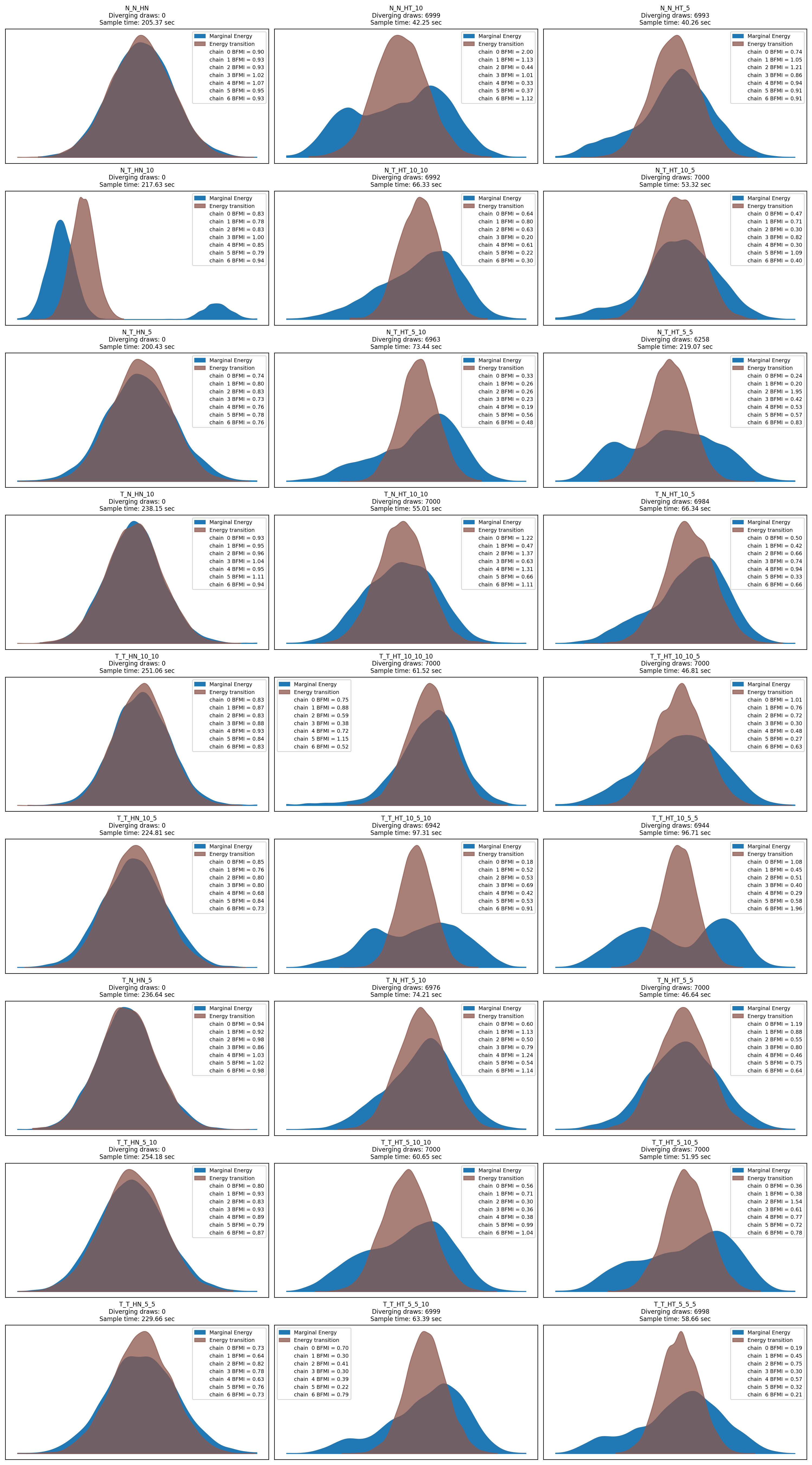

# Combine into InferenceData comparison object
loo_dict = {name: model_traces[name]['scores']['loo'] for name in model_traces.keys()}
cmp_df = az.compare(loo_dict, method="stacking", ic="loo")

# Save the comparison DataFrame
cmp_df.to_csv("../results/model_comparison.csv", )
# Print the comparison DataFrame
print("\nModel Comparison Results:")
cmp_df

Model Comparison Results:

	rank	elpd_loo	p_loo	elpd_diff	weight	se	dse	warning	scale
N_T_HT_5_10	0	-13.942824	112.407689	0.000000	0.501709	26.172102	0.000000	True	log
N_T_HT_10_10	1	-14.232323	115.634082	0.289498	0.232978	25.852563	4.944408	True	log
N_T_HT_10_5	2	-15.196429	113.624439	1.253604	0.265313	25.562472	5.420416	True	log
T_N_HT_10_5	3	-29.299767	103.590498	15.356943	0.000000	26.574965	5.712471	True	log
T_T_HT_10_10_10	4	-30.656224	110.373495	16.713400	0.000000	26.435805	6.042163	True	log
N_T_HT_5_5	5	-33.954243	134.999306	20.011419	0.000000	26.360560	7.147779	True	log
T_N_HT_10_10	6	-39.808868	110.980355	25.866044	0.000000	26.492594	5.556646	True	log
T_T_HT_10_5_5	7	-46.613526	115.610006	32.670702	0.000000	26.806032	6.565634	True	log
T_T_HT_10_10_5	8	-48.198680	120.920450	34.255855	0.000000	26.793137	7.001829	True	log
T_T_HT_5_10_5	9	-59.106328	105.086513	45.163503	0.000000	27.142046	6.035451	True	log
T_T_HT_5_5_5	10	-59.685208	102.204978	45.742384	0.000000	27.823967	7.678840	True	log
T_T_HT_5_10_10	11	-60.728334	102.599512	46.785510	0.000000	27.133034	6.249436	True	log
T_N_HT_5_5	12	-67.525844	107.832978	53.583020	0.000000	27.624499	7.079179	True	log
N_T_HN_10	13	-173.060588	68.185244	159.117764	0.000000	25.601244	7.208652	False	log
N_N_HT_10	14	-174.314027	221.807800	160.371203	0.000000	25.234972	7.764120	True	log
N_N_HT_5	15	-183.304207	230.436980	169.361383	0.000000	25.714858	8.332182	True	log
N_N_HN	16	-190.088696	65.218096	176.145872	0.000000	25.583171	7.596365	False	log
T_T_HN_10_10	17	-192.626419	65.398645	178.683595	0.000000	26.146340	7.334733	False	log
T_T_HT_10_5_10	18	-196.046002	215.026323	182.103178	0.000000	26.522684	6.822517	True	log
T_N_HN_10	19	-208.959314	61.984608	195.016489	0.000000	26.085043	7.693501	False	log
T_T_HN_5_10	20	-216.997040	62.653391	203.054216	0.000000	26.711356	7.740838	False	log
T_N_HT_5_10	21	-229.496264	218.853051	215.553440	0.000000	27.049425	7.853962	True	log
T_T_HT_5_5_10	22	-230.189140	214.764648	216.246316	0.000000	27.201740	7.730539	True	log
T_N_HN_5	23	-233.133380	59.696692	219.190556	0.000000	26.665638	8.054481	False	log
N_T_HN_5	24	-248.998777	58.803980	235.055953	0.000000	25.585742	9.124896	False	log
T_T_HN_10_5	25	-267.526199	56.568757	253.583375	0.000000	26.100456	9.161338	True	log
T_T_HN_5_5	26	-291.694932	54.513089	277.752108	0.000000	26.616132	9.474451	False	log

Import and analyze the results

import pandas as pd
import arviz as az
from pathlib import Path
from cloudpickle import load
from glob import glob

# Load models
model_traces = {}
for pkl in glob("../results/models/*.pkl"):
    name = Path(pkl).name.removesuffix("_model.pkl")
    trace_path = f"../results/traces/{name}_trace.nc"
    model_traces[name] = {}
    with open(pkl, "rb") as f:
        model_traces[name]['model'] = load(f)
    model_traces[name]['trace'] = az.from_netcdf(trace_path)

# Load the comparison DataFrame
cmp_df = pd.read_csv("../results/model_comparison.csv", index_col=0)

az.plot_compare(cmp_df, textsize=8, insample_dev=True);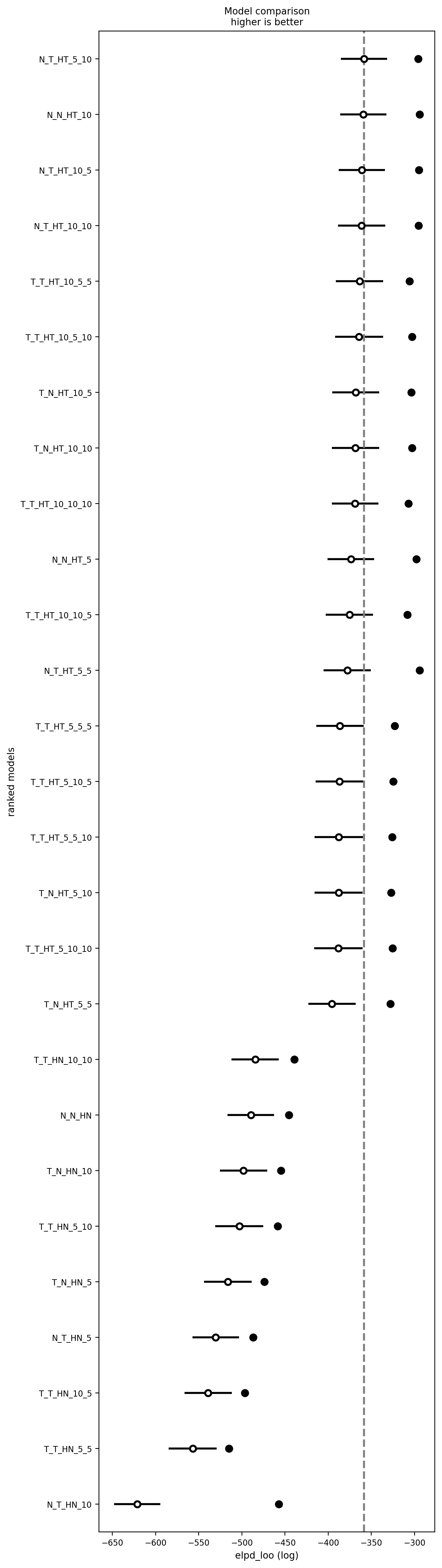

import matplotlib.pyplot as plt

top_n = 8


for name in cmp_df.index[:top_n]:
    f, axs = plt.subplots(1,2, figsize=(12, 3))
    trace = model_traces[name]['trace']
    az.plot_loo_pit(trace, y='y_hat', ax=axs[0])
    az.plot_loo_pit(trace, y='y_hat', ecdf=True, ax=axs[1])
    f.suptitle(f"PIT for {name}")
    f.tight_layout()

/home/sojern/miniconda3/envs/pymc/lib/python3.13/site-packages/arviz/stats/stats.py:1045: RuntimeWarning: overflow encountered in exp
  weights = 1 / np.exp(len_scale - len_scale[:, None]).sum(axis=1)
/home/sojern/miniconda3/envs/pymc/lib/python3.13/site-packages/numpy/_core/_methods.py:52: RuntimeWarning: overflow encountered in reduce
  return umr_sum(a, axis, dtype, out, keepdims, initial, where)
/home/sojern/miniconda3/envs/pymc/lib/python3.13/site-packages/arviz/stats/stats.py:1045: RuntimeWarning: overflow encountered in exp
  weights = 1 / np.exp(len_scale - len_scale[:, None]).sum(axis=1)
/home/sojern/miniconda3/envs/pymc/lib/python3.13/site-packages/numpy/_core/_methods.py:52: RuntimeWarning: overflow encountered in reduce
  return umr_sum(a, axis, dtype, out, keepdims, initial, where)
/home/sojern/miniconda3/envs/pymc/lib/python3.13/site-packages/arviz/stats/stats.py:1045: RuntimeWarning: overflow encountered in exp
  weights = 1 / np.exp(len_scale - len_scale[:, None]).sum(axis=1)
/home/sojern/miniconda3/envs/pymc/lib/python3.13/site-packages/numpy/_core/_methods.py:52: RuntimeWarning: overflow encountered in reduce
  return umr_sum(a, axis, dtype, out, keepdims, initial, where)
/home/sojern/miniconda3/envs/pymc/lib/python3.13/site-packages/arviz/stats/stats.py:1045: RuntimeWarning: overflow encountered in exp
  weights = 1 / np.exp(len_scale - len_scale[:, None]).sum(axis=1)
/home/sojern/miniconda3/envs/pymc/lib/python3.13/site-packages/numpy/_core/_methods.py:52: RuntimeWarning: overflow encountered in reduce
  return umr_sum(a, axis, dtype, out, keepdims, initial, where)
/home/sojern/miniconda3/envs/pymc/lib/python3.13/site-packages/arviz/stats/stats.py:1045: RuntimeWarning: overflow encountered in exp
  weights = 1 / np.exp(len_scale - len_scale[:, None]).sum(axis=1)
/home/sojern/miniconda3/envs/pymc/lib/python3.13/site-packages/numpy/_core/_methods.py:52: RuntimeWarning: overflow encountered in reduce
  return umr_sum(a, axis, dtype, out, keepdims, initial, where)
/home/sojern/miniconda3/envs/pymc/lib/python3.13/site-packages/arviz/stats/stats.py:1045: RuntimeWarning: overflow encountered in exp
  weights = 1 / np.exp(len_scale - len_scale[:, None]).sum(axis=1)
/home/sojern/miniconda3/envs/pymc/lib/python3.13/site-packages/numpy/_core/_methods.py:52: RuntimeWarning: overflow encountered in reduce
  return umr_sum(a, axis, dtype, out, keepdims, initial, where)
/home/sojern/miniconda3/envs/pymc/lib/python3.13/site-packages/arviz/stats/stats.py:1045: RuntimeWarning: overflow encountered in exp
  weights = 1 / np.exp(len_scale - len_scale[:, None]).sum(axis=1)
/home/sojern/miniconda3/envs/pymc/lib/python3.13/site-packages/numpy/_core/_methods.py:52: RuntimeWarning: overflow encountered in reduce
  return umr_sum(a, axis, dtype, out, keepdims, initial, where)
/home/sojern/miniconda3/envs/pymc/lib/python3.13/site-packages/arviz/stats/stats.py:1045: RuntimeWarning: overflow encountered in exp
  weights = 1 / np.exp(len_scale - len_scale[:, None]).sum(axis=1)
/home/sojern/miniconda3/envs/pymc/lib/python3.13/site-packages/numpy/_core/_methods.py:52: RuntimeWarning: overflow encountered in reduce
  return umr_sum(a, axis, dtype, out, keepdims, initial, where)
/home/sojern/miniconda3/envs/pymc/lib/python3.13/site-packages/arviz/stats/stats.py:1045: RuntimeWarning: overflow encountered in exp
  weights = 1 / np.exp(len_scale - len_scale[:, None]).sum(axis=1)
/home/sojern/miniconda3/envs/pymc/lib/python3.13/site-packages/numpy/_core/_methods.py:52: RuntimeWarning: overflow encountered in reduce
  return umr_sum(a, axis, dtype, out, keepdims, initial, where)
/home/sojern/miniconda3/envs/pymc/lib/python3.13/site-packages/arviz/stats/stats.py:1045: RuntimeWarning: overflow encountered in exp
  weights = 1 / np.exp(len_scale - len_scale[:, None]).sum(axis=1)
/home/sojern/miniconda3/envs/pymc/lib/python3.13/site-packages/numpy/_core/_methods.py:52: RuntimeWarning: overflow encountered in reduce
  return umr_sum(a, axis, dtype, out, keepdims, initial, where)
/home/sojern/miniconda3/envs/pymc/lib/python3.13/site-packages/arviz/stats/stats.py:1045: RuntimeWarning: overflow encountered in exp
  weights = 1 / np.exp(len_scale - len_scale[:, None]).sum(axis=1)
/home/sojern/miniconda3/envs/pymc/lib/python3.13/site-packages/numpy/_core/_methods.py:52: RuntimeWarning: overflow encountered in reduce
  return umr_sum(a, axis, dtype, out, keepdims, initial, where)
/home/sojern/miniconda3/envs/pymc/lib/python3.13/site-packages/arviz/stats/stats.py:1045: RuntimeWarning: overflow encountered in exp
  weights = 1 / np.exp(len_scale - len_scale[:, None]).sum(axis=1)
/home/sojern/miniconda3/envs/pymc/lib/python3.13/site-packages/numpy/_core/_methods.py:52: RuntimeWarning: overflow encountered in reduce
  return umr_sum(a, axis, dtype, out, keepdims, initial, where)
/home/sojern/miniconda3/envs/pymc/lib/python3.13/site-packages/arviz/stats/stats.py:1045: RuntimeWarning: overflow encountered in exp
  weights = 1 / np.exp(len_scale - len_scale[:, None]).sum(axis=1)
/home/sojern/miniconda3/envs/pymc/lib/python3.13/site-packages/numpy/_core/_methods.py:52: RuntimeWarning: overflow encountered in reduce
  return umr_sum(a, axis, dtype, out, keepdims, initial, where)
/home/sojern/miniconda3/envs/pymc/lib/python3.13/site-packages/arviz/stats/stats.py:1045: RuntimeWarning: overflow encountered in exp
  weights = 1 / np.exp(len_scale - len_scale[:, None]).sum(axis=1)
/home/sojern/miniconda3/envs/pymc/lib/python3.13/site-packages/numpy/_core/_methods.py:52: RuntimeWarning: overflow encountered in reduce
  return umr_sum(a, axis, dtype, out, keepdims, initial, where)
/home/sojern/miniconda3/envs/pymc/lib/python3.13/site-packages/arviz/stats/stats.py:1045: RuntimeWarning: overflow encountered in exp
  weights = 1 / np.exp(len_scale - len_scale[:, None]).sum(axis=1)
/home/sojern/miniconda3/envs/pymc/lib/python3.13/site-packages/numpy/_core/_methods.py:52: RuntimeWarning: overflow encountered in reduce
  return umr_sum(a, axis, dtype, out, keepdims, initial, where)
/home/sojern/miniconda3/envs/pymc/lib/python3.13/site-packages/arviz/stats/stats.py:1045: RuntimeWarning: overflow encountered in exp
  weights = 1 / np.exp(len_scale - len_scale[:, None]).sum(axis=1)
/home/sojern/miniconda3/envs/pymc/lib/python3.13/site-packages/numpy/_core/_methods.py:52: RuntimeWarning: overflow encountered in reduce
  return umr_sum(a, axis, dtype, out, keepdims, initial, where)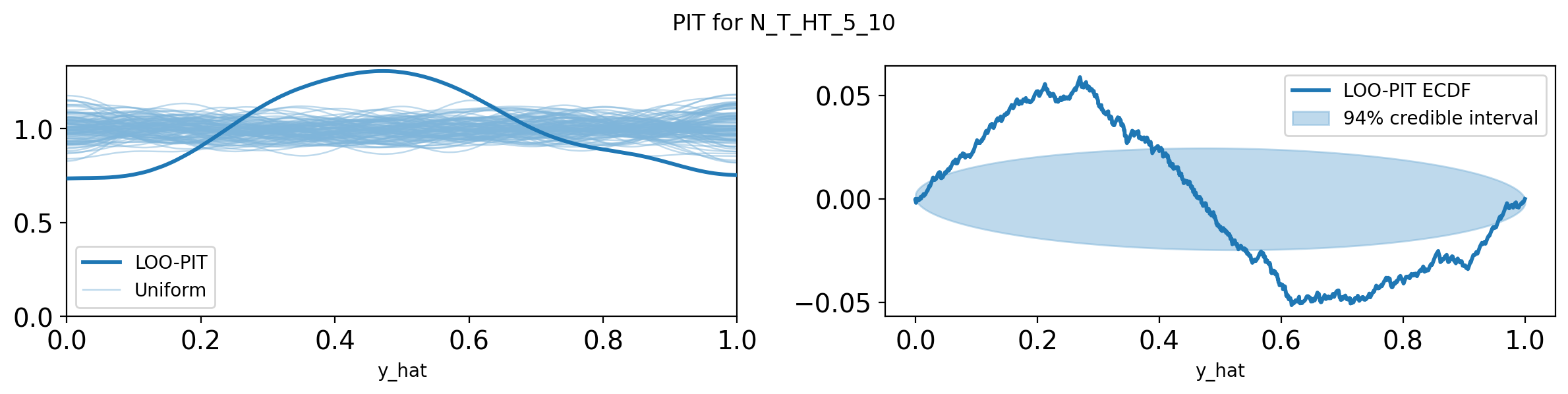

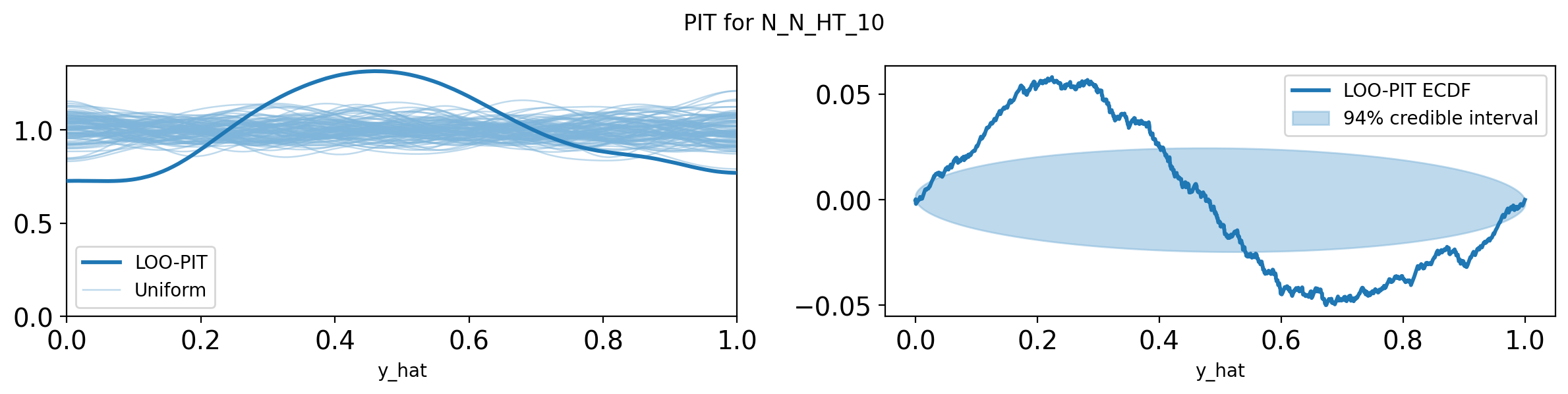
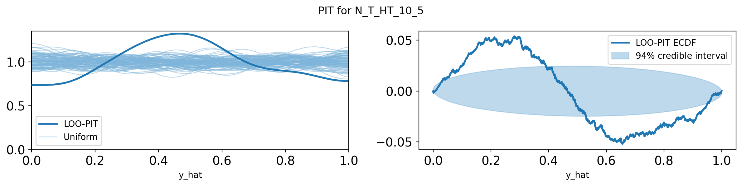
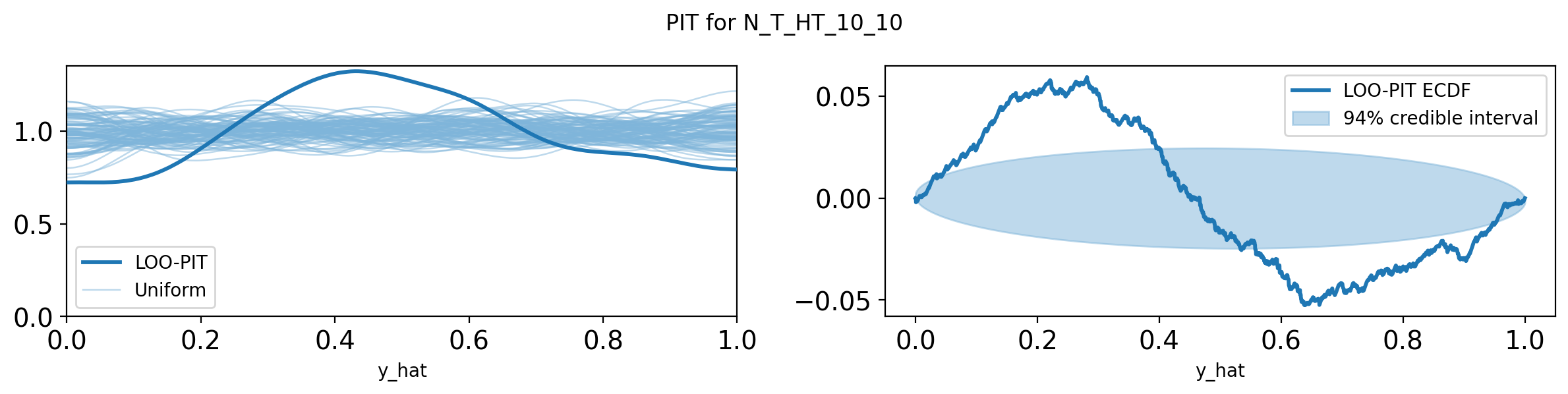
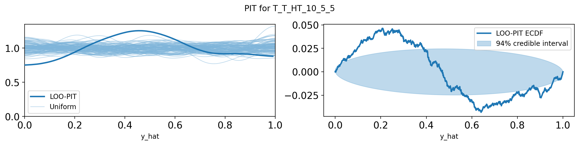
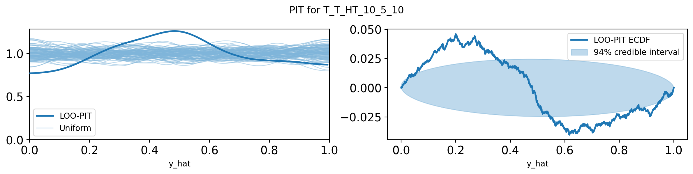
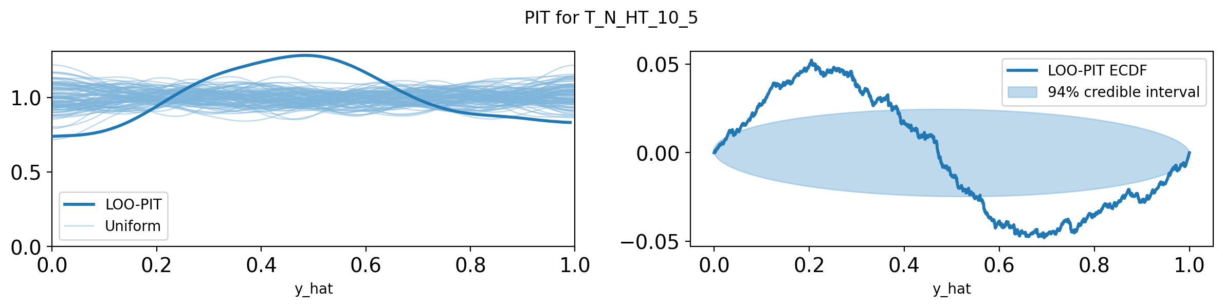
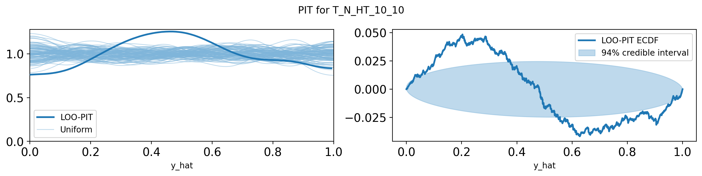
Test: Post-hoc decoding of mixture weight

import arviz as az
import cloudpickle as cp

name = "N_N_HN"

trace = az.from_netcdf(f"../results/traces/{name}_trace.nc")

with open(f"../results/models/{name}_model.pkl", "rb") as f:
    model = cp.load(f)

trace

arviz.InferenceData

• posterior

  <xarray.Dataset> Size: 242MB
  Dimensions:      (chain: 7, draw: 1000, pos: 1438, mu_dim_0: 2, sigma_dim_0: 2)
  Coordinates:
    * chain        (chain) int64 56B 0 1 2 3 4 5 6
    * draw         (draw) int64 8kB 0 1 2 3 4 5 6 ... 993 994 995 996 997 998 999
    * pos          (pos) int64 12kB 24 25 26 27 28 29 ... 1615 1618 1619 1620 1621
    * mu_dim_0     (mu_dim_0) int64 16B 0 1
    * sigma_dim_0  (sigma_dim_0) int64 16B 0 1
  Data variables:
      eps          (chain, draw, pos) float64 81MB ...
      mu           (chain, draw, mu_dim_0) float64 112kB ...
      sigma        (chain, draw, sigma_dim_0) float64 112kB ...
      grw_sigma    (chain, draw) float64 56kB ...
      logit_w      (chain, draw, pos) float64 81MB ...
      w            (chain, draw, pos) float64 81MB ...
  Attributes:
      created_at:                 2025-07-17T20:42:05.061371+00:00
      arviz_version:              0.21.0
      inference_library:          pymc
      inference_library_version:  5.22.0
      sampling_time:              302.33364176750183
      tuning_steps:               1000

  xarray.Dataset

  • Dimensions:
    • chain: 7
    • draw: 1000
    • pos: 1438
    • mu_dim_0: 2
    • sigma_dim_0: 2
  • Coordinates: (5)
    • chain
      (chain)
      int64
      0 1 2 3 4 5 6

      array([0, 1, 2, 3, 4, 5, 6])

    • draw
      (draw)
      int64
      0 1 2 3 4 5 ... 995 996 997 998 999

      array([  0,   1,   2, ..., 997, 998, 999], shape=(1000,))

    • pos
      (pos)
      int64
      24 25 26 27 ... 1618 1619 1620 1621

      array([  24,   25,   26, ..., 1619, 1620, 1621], shape=(1438,))

    • mu_dim_0
      (mu_dim_0)
      int64
      0 1

      array([0, 1])

    • sigma_dim_0
      (sigma_dim_0)
      int64
      0 1

      array([0, 1])

  • Data variables: (6)
    • eps
      (chain, draw, pos)
      float64
      ...

      [10066000 values with dtype=float64]

    • mu
      (chain, draw, mu_dim_0)
      float64
      ...

      [14000 values with dtype=float64]

    • sigma
      (chain, draw, sigma_dim_0)
      float64
      ...

      [14000 values with dtype=float64]

    • grw_sigma
      (chain, draw)
      float64
      ...

      [7000 values with dtype=float64]

    • logit_w
      (chain, draw, pos)
      float64
      ...

      [10066000 values with dtype=float64]

    • w
      (chain, draw, pos)
      float64
      ...

      [10066000 values with dtype=float64]

  • Indexes: (5)
    • chain
      PandasIndex

      PandasIndex(Index([0, 1, 2, 3, 4, 5, 6], dtype='int64', name='chain'))

    • draw
      PandasIndex

      PandasIndex(Index([  0,   1,   2,   3,   4,   5,   6,   7,   8,   9,
             ...
             990, 991, 992, 993, 994, 995, 996, 997, 998, 999],
            dtype='int64', name='draw', length=1000))

    • pos
      PandasIndex

      PandasIndex(Index([  24,   25,   26,   27,   28,   29,   30,   31,   32,   33,
             ...
             1610, 1611, 1612, 1613, 1614, 1615, 1618, 1619, 1620, 1621],
            dtype='int64', name='pos', length=1438))

    • mu_dim_0
      PandasIndex

      PandasIndex(Index([0, 1], dtype='int64', name='mu_dim_0'))

    • sigma_dim_0
      PandasIndex

      PandasIndex(Index([0, 1], dtype='int64', name='sigma_dim_0'))

  • Attributes: (6)

    created_at :

    2025-07-17T20:42:05.061371+00:00

    arviz_version :

    0.21.0

    inference_library :

    pymc

    inference_library_version :

    5.22.0

    sampling_time :

    302.33364176750183

    tuning_steps :

    1000

  
  
• posterior_predictive

  <xarray.Dataset> Size: 81MB
  Dimensions:  (chain: 7, draw: 1000, pos: 1438)
  Coordinates:
    * chain    (chain) int64 56B 0 1 2 3 4 5 6
    * draw     (draw) int64 8kB 0 1 2 3 4 5 6 7 ... 993 994 995 996 997 998 999
    * pos      (pos) int64 12kB 24 25 26 27 28 29 ... 1615 1618 1619 1620 1621
  Data variables:
      y_hat    (chain, draw, pos) float64 81MB ...
  Attributes:
      created_at:                 2025-07-17T22:04:45.542489+00:00
      arviz_version:              0.21.0
      inference_library:          pymc
      inference_library_version:  5.22.0

  xarray.Dataset

  • Dimensions:
    • chain: 7
    • draw: 1000
    • pos: 1438
  • Coordinates: (3)
    • chain
      (chain)
      int64
      0 1 2 3 4 5 6

      array([0, 1, 2, 3, 4, 5, 6])

    • draw
      (draw)
      int64
      0 1 2 3 4 5 ... 995 996 997 998 999

      array([  0,   1,   2, ..., 997, 998, 999], shape=(1000,))

    • pos
      (pos)
      int64
      24 25 26 27 ... 1618 1619 1620 1621

      array([  24,   25,   26, ..., 1619, 1620, 1621], shape=(1438,))

  • Data variables: (1)
    • y_hat
      (chain, draw, pos)
      float64
      ...

      [10066000 values with dtype=float64]

  • Indexes: (3)
    • chain
      PandasIndex

      PandasIndex(Index([0, 1, 2, 3, 4, 5, 6], dtype='int64', name='chain'))

    • draw
      PandasIndex

      PandasIndex(Index([  0,   1,   2,   3,   4,   5,   6,   7,   8,   9,
             ...
             990, 991, 992, 993, 994, 995, 996, 997, 998, 999],
            dtype='int64', name='draw', length=1000))

    • pos
      PandasIndex

      PandasIndex(Index([  24,   25,   26,   27,   28,   29,   30,   31,   32,   33,
             ...
             1610, 1611, 1612, 1613, 1614, 1615, 1618, 1619, 1620, 1621],
            dtype='int64', name='pos', length=1438))

  • Attributes: (4)

    created_at :

    2025-07-17T22:04:45.542489+00:00

    arviz_version :

    0.21.0

    inference_library :

    pymc

    inference_library_version :

    5.22.0

  
  
• log_likelihood

  <xarray.Dataset> Size: 81MB
  Dimensions:  (chain: 7, draw: 1000, pos: 1438)
  Coordinates:
    * chain    (chain) int64 56B 0 1 2 3 4 5 6
    * draw     (draw) int64 8kB 0 1 2 3 4 5 6 7 ... 993 994 995 996 997 998 999
    * pos      (pos) int64 12kB 24 25 26 27 28 29 ... 1615 1618 1619 1620 1621
  Data variables:
      y_hat    (chain, draw, pos) float64 81MB ...
  Attributes:
      created_at:                 2025-07-17T22:04:05.221796+00:00
      arviz_version:              0.21.0
      inference_library:          pymc
      inference_library_version:  5.22.0

  xarray.Dataset

  • Dimensions:
    • chain: 7
    • draw: 1000
    • pos: 1438
  • Coordinates: (3)
    • chain
      (chain)
      int64
      0 1 2 3 4 5 6

      array([0, 1, 2, 3, 4, 5, 6])

    • draw
      (draw)
      int64
      0 1 2 3 4 5 ... 995 996 997 998 999

      array([  0,   1,   2, ..., 997, 998, 999], shape=(1000,))

    • pos
      (pos)
      int64
      24 25 26 27 ... 1618 1619 1620 1621

      array([  24,   25,   26, ..., 1619, 1620, 1621], shape=(1438,))

  • Data variables: (1)
    • y_hat
      (chain, draw, pos)
      float64
      ...

      [10066000 values with dtype=float64]

  • Indexes: (3)
    • chain
      PandasIndex

      PandasIndex(Index([0, 1, 2, 3, 4, 5, 6], dtype='int64', name='chain'))

    • draw
      PandasIndex

      PandasIndex(Index([  0,   1,   2,   3,   4,   5,   6,   7,   8,   9,
             ...
             990, 991, 992, 993, 994, 995, 996, 997, 998, 999],
            dtype='int64', name='draw', length=1000))

    • pos
      PandasIndex

      PandasIndex(Index([  24,   25,   26,   27,   28,   29,   30,   31,   32,   33,
             ...
             1610, 1611, 1612, 1613, 1614, 1615, 1618, 1619, 1620, 1621],
            dtype='int64', name='pos', length=1438))

  • Attributes: (4)

    created_at :

    2025-07-17T22:04:05.221796+00:00

    arviz_version :

    0.21.0

    inference_library :

    pymc

    inference_library_version :

    5.22.0

  
  
• sample_stats

  <xarray.Dataset> Size: 862kB
  Dimensions:                (chain: 7, draw: 1000)
  Coordinates:
    * chain                  (chain) int64 56B 0 1 2 3 4 5 6
    * draw                   (draw) int64 8kB 0 1 2 3 4 5 ... 995 996 997 998 999
  Data variables: (12/17)
      tree_depth             (chain, draw) int64 56kB ...
      largest_eigval         (chain, draw) float64 56kB ...
      step_size_bar          (chain, draw) float64 56kB ...
      process_time_diff      (chain, draw) float64 56kB ...
      diverging              (chain, draw) bool 7kB ...
      step_size              (chain, draw) float64 56kB ...
      ...                     ...
      acceptance_rate        (chain, draw) float64 56kB ...
      index_in_trajectory    (chain, draw) int64 56kB ...
      perf_counter_start     (chain, draw) float64 56kB ...
      max_energy_error       (chain, draw) float64 56kB ...
      lp                     (chain, draw) float64 56kB ...
      perf_counter_diff      (chain, draw) float64 56kB ...
  Attributes:
      created_at:                 2025-07-17T20:42:05.081859+00:00
      arviz_version:              0.21.0
      inference_library:          pymc
      inference_library_version:  5.22.0
      sampling_time:              302.33364176750183
      tuning_steps:               1000

  xarray.Dataset

  • Dimensions:
    • chain: 7
    • draw: 1000
  • Coordinates: (2)
    • chain
      (chain)
      int64
      0 1 2 3 4 5 6

      array([0, 1, 2, 3, 4, 5, 6])

    • draw
      (draw)
      int64
      0 1 2 3 4 5 ... 995 996 997 998 999

      array([  0,   1,   2, ..., 997, 998, 999], shape=(1000,))

  • Data variables: (17)
    • tree_depth
      (chain, draw)
      int64
      ...

      [7000 values with dtype=int64]

    • largest_eigval
      (chain, draw)
      float64
      ...

      [7000 values with dtype=float64]

    • step_size_bar
      (chain, draw)
      float64
      ...

      [7000 values with dtype=float64]

    • process_time_diff
      (chain, draw)
      float64
      ...

      [7000 values with dtype=float64]

    • diverging
      (chain, draw)
      bool
      ...

      [7000 values with dtype=bool]

    • step_size
      (chain, draw)
      float64
      ...

      [7000 values with dtype=float64]

    • reached_max_treedepth
      (chain, draw)
      bool
      ...

      [7000 values with dtype=bool]

    • n_steps
      (chain, draw)
      float64
      ...

      [7000 values with dtype=float64]

    • energy_error
      (chain, draw)
      float64
      ...

      [7000 values with dtype=float64]

    • energy
      (chain, draw)
      float64
      ...

      [7000 values with dtype=float64]

    • smallest_eigval
      (chain, draw)
      float64
      ...

      [7000 values with dtype=float64]

    • acceptance_rate
      (chain, draw)
      float64
      ...

      [7000 values with dtype=float64]

    • index_in_trajectory
      (chain, draw)
      int64
      ...

      [7000 values with dtype=int64]

    • perf_counter_start
      (chain, draw)
      float64
      ...

      [7000 values with dtype=float64]

    • max_energy_error
      (chain, draw)
      float64
      ...

      [7000 values with dtype=float64]

    • lp
      (chain, draw)
      float64
      ...

      [7000 values with dtype=float64]

    • perf_counter_diff
      (chain, draw)
      float64
      ...

      [7000 values with dtype=float64]

  • Indexes: (2)
    • chain
      PandasIndex

      PandasIndex(Index([0, 1, 2, 3, 4, 5, 6], dtype='int64', name='chain'))

    • draw
      PandasIndex

      PandasIndex(Index([  0,   1,   2,   3,   4,   5,   6,   7,   8,   9,
             ...
             990, 991, 992, 993, 994, 995, 996, 997, 998, 999],
            dtype='int64', name='draw', length=1000))

  • Attributes: (6)

    created_at :

    2025-07-17T20:42:05.081859+00:00

    arviz_version :

    0.21.0

    inference_library :

    pymc

    inference_library_version :

    5.22.0

    sampling_time :

    302.33364176750183

    tuning_steps :

    1000

  
  
• prior

  <xarray.Dataset> Size: 35MB
  Dimensions:      (chain: 1, draw: 1000, pos: 1438, sigma_dim_0: 2, mu_dim_0: 2)
  Coordinates:
    * chain        (chain) int64 8B 0
    * draw         (draw) int64 8kB 0 1 2 3 4 5 6 ... 993 994 995 996 997 998 999
    * pos          (pos) int64 12kB 24 25 26 27 28 29 ... 1615 1618 1619 1620 1621
    * sigma_dim_0  (sigma_dim_0) int64 16B 0 1
    * mu_dim_0     (mu_dim_0) int64 16B 0 1
  Data variables:
      grw_sigma    (chain, draw) float64 8kB ...
      w            (chain, draw, pos) float64 12MB ...
      sigma        (chain, draw, sigma_dim_0) float64 16kB ...
      eps          (chain, draw, pos) float64 12MB ...
      logit_w      (chain, draw, pos) float64 12MB ...
      mu           (chain, draw, mu_dim_0) float64 16kB ...
  Attributes:
      created_at:                 2025-07-17T22:04:10.448419+00:00
      arviz_version:              0.21.0
      inference_library:          pymc
      inference_library_version:  5.22.0

  xarray.Dataset

  • Dimensions:
    • chain: 1
    • draw: 1000
    • pos: 1438
    • sigma_dim_0: 2
    • mu_dim_0: 2
  • Coordinates: (5)
    • chain
      (chain)
      int64
      0

      array([0])

    • draw
      (draw)
      int64
      0 1 2 3 4 5 ... 995 996 997 998 999

      array([  0,   1,   2, ..., 997, 998, 999], shape=(1000,))

    • pos
      (pos)
      int64
      24 25 26 27 ... 1618 1619 1620 1621

      array([  24,   25,   26, ..., 1619, 1620, 1621], shape=(1438,))

    • sigma_dim_0
      (sigma_dim_0)
      int64
      0 1

      array([0, 1])

    • mu_dim_0
      (mu_dim_0)
      int64
      0 1

      array([0, 1])

  • Data variables: (6)
    • grw_sigma
      (chain, draw)
      float64
      ...

      [1000 values with dtype=float64]

    • w
      (chain, draw, pos)
      float64
      ...

      [1438000 values with dtype=float64]

    • sigma
      (chain, draw, sigma_dim_0)
      float64
      ...

      [2000 values with dtype=float64]

    • eps
      (chain, draw, pos)
      float64
      ...

      [1438000 values with dtype=float64]

    • logit_w
      (chain, draw, pos)
      float64
      ...

      [1438000 values with dtype=float64]

    • mu
      (chain, draw, mu_dim_0)
      float64
      ...

      [2000 values with dtype=float64]

  • Indexes: (5)
    • chain
      PandasIndex

      PandasIndex(Index([0], dtype='int64', name='chain'))

    • draw
      PandasIndex

      PandasIndex(Index([  0,   1,   2,   3,   4,   5,   6,   7,   8,   9,
             ...
             990, 991, 992, 993, 994, 995, 996, 997, 998, 999],
            dtype='int64', name='draw', length=1000))

    • pos
      PandasIndex

      PandasIndex(Index([  24,   25,   26,   27,   28,   29,   30,   31,   32,   33,
             ...
             1610, 1611, 1612, 1613, 1614, 1615, 1618, 1619, 1620, 1621],
            dtype='int64', name='pos', length=1438))

    • sigma_dim_0
      PandasIndex

      PandasIndex(Index([0, 1], dtype='int64', name='sigma_dim_0'))

    • mu_dim_0
      PandasIndex

      PandasIndex(Index([0, 1], dtype='int64', name='mu_dim_0'))

  • Attributes: (4)

    created_at :

    2025-07-17T22:04:10.448419+00:00

    arviz_version :

    0.21.0

    inference_library :

    pymc

    inference_library_version :

    5.22.0

  
  
• prior_predictive

  <xarray.Dataset> Size: 12MB
  Dimensions:  (chain: 1, draw: 1000, pos: 1438)
  Coordinates:
    * chain    (chain) int64 8B 0
    * draw     (draw) int64 8kB 0 1 2 3 4 5 6 7 ... 993 994 995 996 997 998 999
    * pos      (pos) int64 12kB 24 25 26 27 28 29 ... 1615 1618 1619 1620 1621
  Data variables:
      y_hat    (chain, draw, pos) float64 12MB ...
  Attributes:
      created_at:                 2025-07-17T22:04:10.455784+00:00
      arviz_version:              0.21.0
      inference_library:          pymc
      inference_library_version:  5.22.0

  xarray.Dataset

  • Dimensions:
    • chain: 1
    • draw: 1000
    • pos: 1438
  • Coordinates: (3)
    • chain
      (chain)
      int64
      0

      array([0])

    • draw
      (draw)
      int64
      0 1 2 3 4 5 ... 995 996 997 998 999

      array([  0,   1,   2, ..., 997, 998, 999], shape=(1000,))

    • pos
      (pos)
      int64
      24 25 26 27 ... 1618 1619 1620 1621

      array([  24,   25,   26, ..., 1619, 1620, 1621], shape=(1438,))

  • Data variables: (1)
    • y_hat
      (chain, draw, pos)
      float64
      ...

      [1438000 values with dtype=float64]

  • Indexes: (3)
    • chain
      PandasIndex

      PandasIndex(Index([0], dtype='int64', name='chain'))

    • draw
      PandasIndex

      PandasIndex(Index([  0,   1,   2,   3,   4,   5,   6,   7,   8,   9,
             ...
             990, 991, 992, 993, 994, 995, 996, 997, 998, 999],
            dtype='int64', name='draw', length=1000))

    • pos
      PandasIndex

      PandasIndex(Index([  24,   25,   26,   27,   28,   29,   30,   31,   32,   33,
             ...
             1610, 1611, 1612, 1613, 1614, 1615, 1618, 1619, 1620, 1621],
            dtype='int64', name='pos', length=1438))

  • Attributes: (4)

    created_at :

    2025-07-17T22:04:10.455784+00:00

    arviz_version :

    0.21.0

    inference_library :

    pymc

    inference_library_version :

    5.22.0

  
  
• observed_data

  <xarray.Dataset> Size: 23kB
  Dimensions:  (pos: 1438)
  Coordinates:
    * pos      (pos) int64 12kB 24 25 26 27 28 29 ... 1615 1618 1619 1620 1621
  Data variables:
      y_hat    (pos) float64 12kB ...
  Attributes:
      created_at:                 2025-07-17T20:42:05.086062+00:00
      arviz_version:              0.21.0
      inference_library:          pymc
      inference_library_version:  5.22.0

  xarray.Dataset

  • Dimensions:
    • pos: 1438
  • Coordinates: (1)
    • pos
      (pos)
      int64
      24 25 26 27 ... 1618 1619 1620 1621

      array([  24,   25,   26, ..., 1619, 1620, 1621], shape=(1438,))

  • Data variables: (1)
    • y_hat
      (pos)
      float64
      ...

      [1438 values with dtype=float64]

  • Indexes: (1)
    • pos
      PandasIndex

      PandasIndex(Index([  24,   25,   26,   27,   28,   29,   30,   31,   32,   33,
             ...
             1610, 1611, 1612, 1613, 1614, 1615, 1618, 1619, 1620, 1621],
            dtype='int64', name='pos', length=1438))

  • Attributes: (4)

    created_at :

    2025-07-17T20:42:05.086062+00:00

    arviz_version :

    0.21.0

    inference_library :

    pymc

    inference_library_version :

    5.22.0

  
  

model

\[ \begin{array}{rcl} \text{mu} &\sim & \operatorname{Normal}(\text{<constant>},~0.3)\\\text{sigma} &\sim & \operatorname{HalfNormal}(0,~0.3)\\\text{grw\_sigma} &\sim & \operatorname{HalfNormal}(0,~0.05)\\\text{eps} &\sim & \operatorname{Normal}(0,~1)\\\text{logit\_w} &\sim & \operatorname{Deterministic}(f(\text{eps},~\text{grw\_sigma}))\\\text{w} &\sim & \operatorname{Deterministic}(f(\text{eps},~\text{grw\_sigma}))\\\text{y\_hat} &\sim & \operatorname{MarginalMixture}(f(\text{eps},~\text{grw\_sigma}),~\operatorname{Normal}(\text{mu},~\text{sigma}))\\\text{y\_hat} &\sim & \operatorname{MarginalMixture}(f(\text{eps},~\text{grw\_sigma}),~\operatorname{Normal}(\text{mu},~\text{sigma})) \end{array} \]

# Just check what the xarray dims look like
trace.posterior['w'].stack(dims=['chain', 'draw'])

<xarray.DataArray 'w' (pos: 1438, dims: 7000)> Size: 81MB
array([[0.44937833, 0.58546809, 0.43819027, ..., 0.51989126, 0.41636437,
        0.43202614],
       [0.52977449, 0.62375669, 0.58263025, ..., 0.50868668, 0.50093716,
        0.5130883 ],
       [0.5916006 , 0.76048527, 0.67466505, ..., 0.70195694, 0.43678679,
        0.44905003],
       ...,
       [0.80690199, 0.73596005, 0.43482456, ..., 0.70743037, 0.26833616,
        0.3913885 ],
       [0.8867993 , 0.56482857, 0.4902178 , ..., 0.77131705, 0.24841057,
        0.35699746],
       [0.82271155, 0.61978168, 0.47971009, ..., 0.77320498, 0.2004193 ,
        0.30180627]], shape=(1438, 7000))
Coordinates:
  * pos      (pos) int64 12kB 24 25 26 27 28 29 ... 1615 1618 1619 1620 1621
  * dims     (dims) object 56kB MultiIndex
  * chain    (dims) int64 56kB 0 0 0 0 0 0 0 0 0 0 0 0 ... 6 6 6 6 6 6 6 6 6 6 6
  * draw     (dims) int64 56kB 0 1 2 3 4 5 6 7 ... 993 994 995 996 997 998 999

xarray.DataArray

'w'

• pos: 1438
• dims: 7000

• 0.4494 0.5855 0.4382 0.6208 0.705 ... 0.5052 0.7732 0.2004 0.3018

  array([[0.44937833, 0.58546809, 0.43819027, ..., 0.51989126, 0.41636437,
          0.43202614],
         [0.52977449, 0.62375669, 0.58263025, ..., 0.50868668, 0.50093716,
          0.5130883 ],
         [0.5916006 , 0.76048527, 0.67466505, ..., 0.70195694, 0.43678679,
          0.44905003],
         ...,
         [0.80690199, 0.73596005, 0.43482456, ..., 0.70743037, 0.26833616,
          0.3913885 ],
         [0.8867993 , 0.56482857, 0.4902178 , ..., 0.77131705, 0.24841057,
          0.35699746],
         [0.82271155, 0.61978168, 0.47971009, ..., 0.77320498, 0.2004193 ,
          0.30180627]], shape=(1438, 7000))

• Coordinates: (4)
  • pos
    (pos)
    int64
    24 25 26 27 ... 1618 1619 1620 1621

    array([  24,   25,   26, ..., 1619, 1620, 1621], shape=(1438,))

  • dims
    (dims)
    object
    MultiIndex

    array([(0, 0), (0, 1), (0, 2), ..., (6, 997), (6, 998), (6, 999)],
          shape=(202,), dtype=object)

  • chain
    (dims)
    int64
    0 0 0 0 0 0 0 0 ... 6 6 6 6 6 6 6 6

    array([0, 0, 0, ..., 6, 6, 6], shape=(202,))

  • draw
    (dims)
    int64
    0 1 2 3 4 5 ... 995 996 997 998 999

    array([  0,   1,   2, ..., 997, 998, 999], shape=(202,))

• Indexes: (2)
  • pos
    PandasIndex

    PandasIndex(Index([  24,   25,   26,   27,   28,   29,   30,   31,   32,   33,
           ...
           1610, 1611, 1612, 1613, 1614, 1615, 1618, 1619, 1620, 1621],
          dtype='int64', name='pos', length=1438))

  • dims
    chain
    draw
    PandasMultiIndex

    PandasIndex(MultiIndex([(0,   0),
                (0,   1),
                (0,   2),
                (0,   3),
                (0,   4),
                (0,   5),
                (0,   6),
                (0,   7),
                (0,   8),
                (0,   9),
                ...
                (6, 990),
                (6, 991),
                (6, 992),
                (6, 993),
                (6, 994),
                (6, 995),
                (6, 996),
                (6, 997),
                (6, 998),
                (6, 999)],
               name='dims', length=7000))

• Attributes: (0)

Now, we can flatten the weights to a n_chains*ndraws X n_bins array and assign an underlying distribution with a Bernoulli trial on each draw.

Note, that the mean of the Bernoulli samples from the posterior draws will converge towards the posterior mean of w. It is thus only an unnecessary step that adds noise and not addition information.

import numpy as np

# Extract posterior samples of w
w_flat = trace.posterior['w'].stack(dims=['chain', 'draw'])
w_mean = trace.posterior['w'].mean(dim=['chain', 'draw'])

# Sample z draws
seed = 42
rng = np.random.default_rng(seed)
z_samples = rng.binomial(1, w_flat)   # shape (samples, pos)

# Compute posterior probability of z=1
z_probs = z_samples.mean(axis=1)     # per-position probability

z_samples

array([[1, 1, 1, ..., 1, 1, 1],
       [0, 0, 0, ..., 1, 1, 1],
       [1, 1, 0, ..., 0, 1, 0],
       ...,
       [1, 1, 1, ..., 1, 0, 0],
       [1, 0, 0, ..., 0, 0, 0],
       [1, 1, 0, ..., 1, 1, 0]], shape=(1438, 7000))

z_probs

# Plots as a quick curve
plt.plot(z_probs, color='black', label='Posterior Probability of z=1')
plt.plot(w_mean, color='tab:orange', label='Posterior Mean of w', alpha = 0.5)
plt.hlines([0.95,0.05], xmin=0, xmax=len(z_probs), colors='gray', linestyles='--', label='95% CI');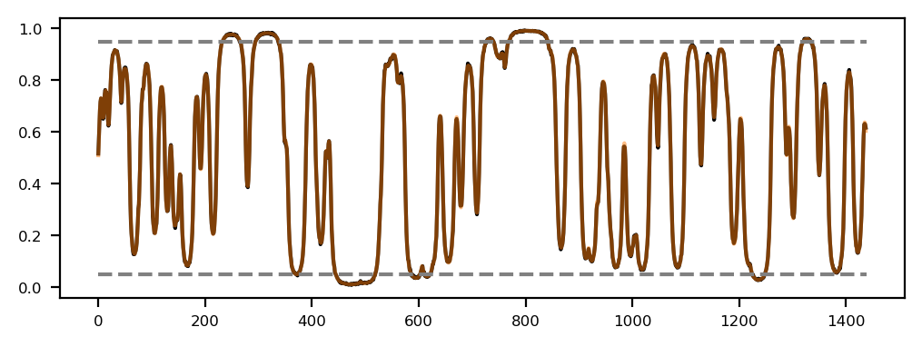

Try some other logic:

# Logic: We define the threshold for a certain assignment of either 
# A: z_posterior > A_threshold,  or B: z_posterior < B_threshold
# The rest will be considered in-transition and could be visualized as a gradient or with shaded regions
A_threshold = 0.05 # A = 0 in the binary assignment
B_threshold = 0.95 # B = 1 in the binary assignment

# Assign compartments based on the threshold
z_assignment = np.where(z_probs < A_threshold, 0, 
                        np.where(z_probs > B_threshold, 1, np.nan))

# Turn around the assignment to have 1 for A and -1 for B
z_assignment = np.where(z_assignment == 0, 1, 
                        np.where(z_assignment == 1, -1, np.nan))

# Plot as quick curve

plt.plot(z_assignment, color='tab:purple', label='Posterior Probability of z=1')
plt.hlines([0.95,0.05], xmin=0, xmax=len(z_assignment), colors='gray', linestyles='--', label='95% CI');

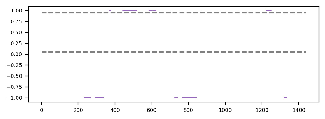
import pandas as pd
import matplotlib.pyplot as plt
import matplotlib_inline
from matplotlib.collections import PatchCollection
from matplotlib.patches import Rectangle

matplotlib_inline.backend_inline.set_matplotlib_formats('svg')

# Load the data
resolution = 100000

y = pd.Series(pd.read_csv(f"../data/eigs/fibroblast.eigs.{resolution}.cis.vecs.tsv", sep="\t")['E1'].values.flatten())
x = pd.Series(np.arange(0,y.shape[0])*resolution)

# Make a DataFrame object
df = pd.DataFrame({"start": x, "e1": y})
df.dropna(inplace=True)


# Quick Plot:
fig, ax = plt.subplots(figsize=(10, 3))
ax.fill_between(df.start, df.e1, where=df.e1 > 0, color='tab:red', ec='None', label='A', step='pre')
ax.fill_between(df.start, df.e1, where=df.e1 < 0, color='tab:blue', ec='None', label='B', step='pre')
ax.plot(df.start, z_assignment, color='tab:green', lw=1, label='z assignment')

# Add shaded areas for the nans
patches = []
in_nan = False
start = None

for i in range(len(z_assignment)):
    if np.isnan(z_assignment[i]) and not in_nan:
        # Start of NaN block
        in_nan = True
        start = df.start.iloc[i]
    elif not np.isnan(z_assignment[i]) and in_nan:
        # End of NaN block
        end = df.start.iloc[i]
        patches.append(Rectangle((start, -1), end - start, 2, alpha=0.2, color='gray'))
        in_nan = False

# If ending on NaNs
if in_nan:
    end = df.start.iloc[-1] + resolution
    patches.append(Rectangle((start, -1), end - start, 2, alpha=1, color='gray'))

ax.add_collection(PatchCollection(patches, match_original=True))


ax.set_xlabel("Genomic Position")
ax.set_ylabel("E1")
ax.legend(loc='lower right')
plt.tight_layout()

---------------------------------------------------------------------------
ValueError                                Traceback (most recent call last)
Cell In[26], line 24
     22 ax.fill_between(df.start, df.e1, where=df.e1 > 0, color='tab:red', ec='None', label='A', step='pre')
     23 ax.fill_between(df.start, df.e1, where=df.e1 < 0, color='tab:blue', ec='None', label='B', step='pre')
---> 24 ax.plot(df.start, z_assignment, color='tab:green', lw=1, label='z assignment')
     26 # Add shaded areas for the nans
     27 patches = []

File ~/miniconda3/envs/pymc/lib/python3.13/site-packages/matplotlib/axes/_axes.py:1777, in Axes.plot(self, scalex, scaley, data, *args, **kwargs)
   1534 """
   1535 Plot y versus x as lines and/or markers.
   1536 
   (...)   1774 (``'green'``) or hex strings (``'#008000'``).
   1775 """
   1776 kwargs = cbook.normalize_kwargs(kwargs, mlines.Line2D)
-> 1777 lines = [*self._get_lines(self, *args, data=data, **kwargs)]
   1778 for line in lines:
   1779     self.add_line(line)

File ~/miniconda3/envs/pymc/lib/python3.13/site-packages/matplotlib/axes/_base.py:297, in _process_plot_var_args.__call__(self, axes, data, return_kwargs, *args, **kwargs)
    295     this += args[0],
    296     args = args[1:]
--> 297 yield from self._plot_args(
    298     axes, this, kwargs, ambiguous_fmt_datakey=ambiguous_fmt_datakey,
    299     return_kwargs=return_kwargs
    300 )

File ~/miniconda3/envs/pymc/lib/python3.13/site-packages/matplotlib/axes/_base.py:494, in _process_plot_var_args._plot_args(self, axes, tup, kwargs, return_kwargs, ambiguous_fmt_datakey)
    491     axes.yaxis.update_units(y)
    493 if x.shape[0] != y.shape[0]:
--> 494     raise ValueError(f"x and y must have same first dimension, but "
    495                      f"have shapes {x.shape} and {y.shape}")
    496 if x.ndim > 2 or y.ndim > 2:
    497     raise ValueError(f"x and y can be no greater than 2D, but have "
    498                      f"shapes {x.shape} and {y.shape}")

ValueError: x and y must have same first dimension, but have shapes (1460,) and (1438,)