import pandas as pd
import numpy as np
import matplotlib.pyplot as plt
import pymc as pm
import arviz as az
from scipy.stats import norm


%config InlineBackend.figure_format = 'retina'
Independent Probabilistic A/B calls
Testing probabilistic modeling of E1 into A/B calls on low-res data with independent bins
Probabilistic Modeling of A/B Compartments from E1
This model infers A/B chromatin compartment structure from the first eigenvector (E1) of the Hi-C contact matrix using a Bayesian framework.
Goals
- Replace hard sign-thresholding of E1 with a probabilistic compartment assignment.
- Quantify uncertainty in compartment calls for each genomic bin.
- Allow for modeling of missing E1 values due to low signal.
Assumptions
- Each bin belongs to one of two latent states: A or B compartment.
- E1 values are generated from Gaussian distributions specific to each compartment.
- Prior belief: A has positive E1 values (μ ≈ 0.5), B has negative (μ ≈ -0.5).
- Bins are initially treated as independent
- Spatial depency can be added later (HMM)
The data
# Input: csv file with only the E1 columns

# Low res example
resolution = 100000

y = pd.Series(pd.read_csv(f"../data/eigs/sperm.eigs.{resolution}.cis.vecs.tsv", sep="\t")['E1'].values.flatten())
bins = np.arange(0, y.shape[0])
x = pd.Series(bins*resolution)

# Make a DataFrame object
df = pd.DataFrame({"bin": bins,
                   "start": x,
                   "e1": y})
df.set_index("bin", inplace=True)

df.dropna(inplace=True)

display(df)| start | e1 | |
|---|---|---|
| bin | ||
| 24 | 2400000 | 0.341686 |
| 25 | 2500000 | 0.335640 |
| 26 | 2600000 | -0.435006 |
| 27 | 2700000 | -0.730504 |
| 28 | 2800000 | -0.908259 |
| ... | ... | ... |
| 1615 | 161500000 | -0.495278 |
| 1618 | 161800000 | -0.428470 |
| 1619 | 161900000 | -0.555748 |
| 1620 | 162000000 | -0.413804 |
| 1621 | 162100000 | 0.013864 |
1438 rows × 2 columns
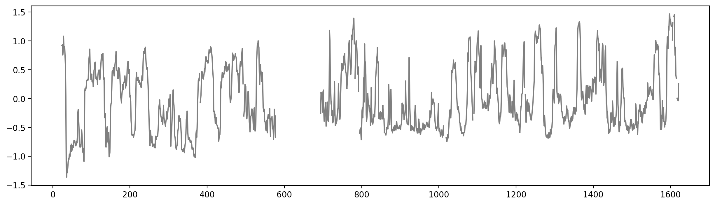
# Plot the data as a track (stairs for niceity)

fig, ax = plt.subplots(figsize=(15, 3))

x_stair = np.zeros(2*y.shape[0])
y_stair = np.zeros(2*y.shape[0])
x_stair[0::2] = x
x_stair[1::2] = x + resolution
y_stair[0::2] = y
y_stair[1::2] = y

ax.fill_between(x_stair, y_stair, where=(y_stair<0), color="tab:blue", ec='None')
ax.fill_between(x_stair, y_stair, where=(y_stair>0), color="tab:red", ec='None')

ax.set_xlim(0, df["start"].max()+resolution)
ticks = np.linspace(0, df["start"].max()+resolution, num=10)
ax.set_xticks(ticks)
ax.set_xticklabels(np.round(ticks / 1e6, 1), rotation=45)
ax.set_xlabel("Genomic Position (Mbp)")
ax.set_ylabel("E1")
ax.set_title("E1");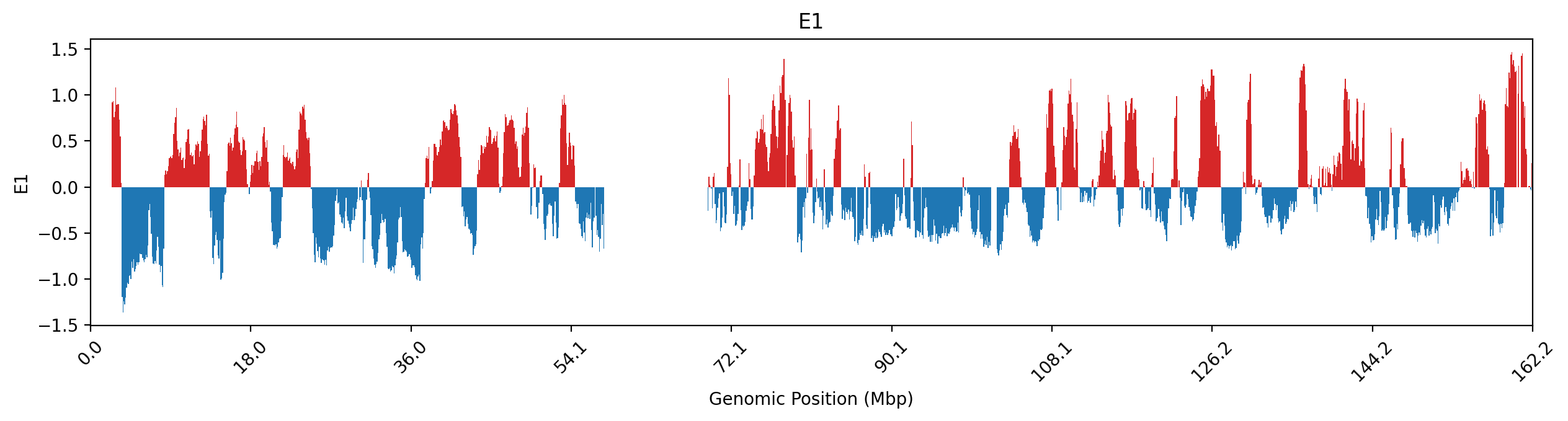
# Histogram of distribution of E1 values (A and B)

f, ax = plt.subplots(figsize=(13, 3))

# A compartments
ax.hist(y[y>0], bins=100, color="tab:red", alpha=0.5, label="A", density=True)
# B compartments
ax.hist(y[y<0], bins=100, color="tab:blue", alpha=0.5, label="B", density=True)
# Mean values (vline)
ax.axvline(y[y>0].mean(), color="tab:red", linestyle="--", label="Mean A")
ax.axvline(y[y<0].mean(), color="tab:blue", linestyle="--", label="Mean B")

# Plot the normal distributions
x_values = np.linspace(y.min(), y.max(), 1000)
mean_a = y[y>0].median()
mean_b = y[y<0].median()
std_a = y[y>0].std()
std_b = y[y<0].std()


ax.plot(x_values, norm.pdf(x_values, loc=mean_a, scale=std_a), color="tab:red", label="Normal A")
ax.plot(x_values, norm.pdf(x_values, loc=mean_b, scale=std_b), color="tab:blue", label="Normal B")
stacked = norm.pdf(x_values, loc=mean_a, scale=std_a) + norm.pdf(x_values, loc=mean_b, scale=std_b)
ax.plot(x_values, stacked, color="tab:purple", label="Stacked Normals")

plt.xlabel("E1")
plt.ylabel("Count")
plt.legend(loc='upper left')
plt.tight_layout()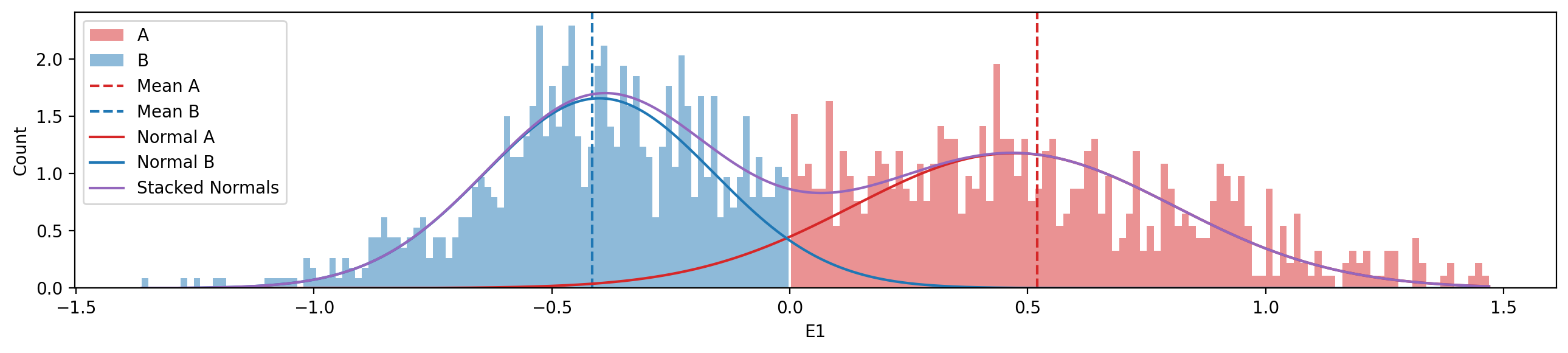
Model Specification
Before specifying the model, we need to layout the model structure.
The model is a mixture of two Gaussian distributions, one for each compartment (A and B). Then a latent variable indicates the compartment assignment for each bin. More formally;
Description
We aim to model the A/B chromatin compartments using a probabilistic generative approach, rather than relying on deterministic eigenvector sign thresholding. Each genomic bin is modeled as belonging to one of two latent states (A or B), with corresponding expected E1 values.
Notation
Let:
- \(y_i\): Observed E1 value at bin \(i\)
- \(z_i \in \{0, 1\}\): Latent compartment assignment (0 = B, 1 = A)
- \(\mu_A, \mu_B\): Mean E1 values for compartments A and B
- \(\sigma\): Shared standard deviation across bins
- \(p\): Prior probability of a bin belonging to compartment A
Model variables
\[ \begin{aligned} \mu_A &\sim \mathcal{N}(0.5, 0.5) \\ \mu_B &\sim \mathcal{N}(-0.5, 0.5) \\ \sigma &\sim \text{HalfNormal}(1) \\ p &\sim \text{Beta}(a, b) \quad \text{(e.g., } a = 2, b = 2 \text{ or something bimodal)} \\ z_i &\sim \text{Bernoulli}(p) \\ \mu_i &= z_i \cdot \mu_A + (1 - z_i) \cdot \mu_B \\ y_i &\sim \mathcal{N}(\mu_i, \sigma) \\ \end{aligned} \]
This model allows us to infer both the compartment state and the uncertainty of the assignment, especially around boundaries between A and B compartments.
The Priors
- \(\mu_A\) and \(\mu_B\): We assume that the mean E1 values for compartments A and B are normally distributed around 0.5 and -0.5, respectively, with a standard deviation of 0.5. This reflects our prior belief about the expected E1 values for each compartment.
- \(\sigma\): The standard deviation is modeled using a half-normal distribution, which ensures that it is always positive. This allows for flexibility in modeling the variability of E1 values within each compartment.
- \(p\): The prior probability of a bin belonging to compartment A is modeled using a Beta distribution. This allows us to incorporate prior beliefs about the expected proportion of bins in each compartment. The parameters \(a\) and \(b\) can be adjusted to reflect different prior beliefs (e.g., bimodal distributions).
- \(z_i\): The latent variable indicating the compartment assignment for each bin is modeled using a Bernoulli distribution, with the probability of being in compartment A given by \(p\).
- \(y_i\): The observed E1 values are modeled as normally distributed around the mean E1 value for the assigned compartment, with a shared standard deviation \(\sigma\). This generative model allows us to infer the compartment assignments and their associated uncertainties based on the observed E1 values, while also accounting for the variability in the data.
Let’s look at a few different options for the Beta distribution. There are 3 main options:
- Uniform: \(a = 1, b = 1\) (no prior preference for A or B)
- Bimodal: \(a = 0.5, b = 0.5\) (most observations are certain to belong to A or B, but a few observations are hard to categorize—borders)
- Unimodal: \(a = 2, b = 2\) (most obsevations are hard to categorize)
Here, they are visualized:
# First, have a look at different Beta distributions for the prior on the latent state (z)

fig, ax = plt.subplots()

params = [(0.5, 0.5), (2, 2), (1, 1)]
colors = ["tab:blue", "tab:orange", "tab:green"]

for (a, b),col in zip(params, colors):
    with pm.Model() as model:
        p = pm.Beta("p", alpha=a, beta=b)
        prior = pm.sample_prior_predictive(samples=10000)
        az.plot_kde(prior.prior["p"].values, label=f"Beta({a}, {b})", ax=ax, fill_kwargs={"alpha": 0.2, "color":col})

ax.set_title("Comparison of Beta priors for p")
ax.set_xlabel("p")
ax.set_ylabel("Density")
ax.legend()
plt.show()
Sampling: [p]
Sampling: [p]
Sampling: [p]
~~I find that the most useful prior is the bimodal one, as we have a strong prior belief that most bins are either A or B, but a few bins are hard to categorize. This is especially useful for the edges of compartments, where the E1 values are close to 0. The unimodal prior is not very useful, as it assumes that most bins are hard to categorize, which is not the case in our data. The uniform prior could be useful as the most uninformative prior —the least biased.*~~
Above logic is flawed. This is not what the prior is reflecting. A Beta(0.5, 0.5) prior assumes that a data set is most likely consisting of only A or B compartments. Therefore, we need Beta(2,2) to reflect that compartments are expected to of both A and B.
fig, ax = plt.subplots((2))

#params = [(0.5, 0.5), (2, 2), (1, 1)]
params = [(1,0), (3,0), (5,0)]
colors = ["tab:blue", "tab:orange", "tab:green"]

for (a, b),col in zip(params, colors):
    with pm.Model() as ylik_priors:
        nu_norm = pm.HalfNormal("nu_norm", sigma=a)
        nu_exp = pm.Exponential("nu_exp", lam=a)
        prior = pm.sample_prior_predictive(samples=10000)
        ax[0].set_title("Comparison of HalfNormal priors for nu")
        az.plot_kde(prior.prior["nu_norm"].values, label=f"HalfN(sigma={a})", ax=ax[0], fill_kwargs={"alpha": 0.2, "color":col})
        ax[1].set_title("Comparison of Exponential priors for nu")
        az.plot_kde(prior.prior["nu_exp"].values, label=f"Exp(lam={a})", ax=ax[1], fill_kwargs={"alpha": 0.2, "color":col})

plt.tight_layout()
Sampling: [nu_exp, nu_norm]
Sampling: [nu_exp, nu_norm]
Sampling: [nu_exp, nu_norm]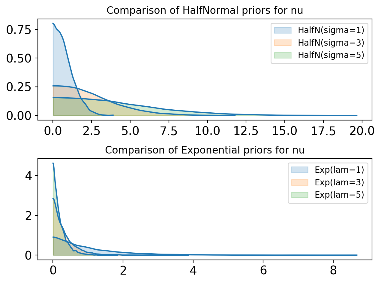
Model in PyMC
coords = {"bins": df.index.values,
          "pos": df.start.values}

with pm.Model(coords=coords) as model:
    # Let the model be aware of the data
    ## Cannot be done with missing values or masked arrays
    # e1 = pm.Data("e1", df.e1.values, dims="bins")

    # Two means for A and B compartments
    mu_a = pm.Normal("mu_a", 0.5, 0.3)
    mu_b = pm.Normal("mu_b", -0.5, 0.3)

    # Standard deviation for the noise (only positive values HalfStudent)
    sigma = pm.HalfNormal("sigma", 0.3)

    # Latent state for each bin: 1 = A, 0 = B
    p = pm.Beta("p", 2, 2, dims="pos")

    # Latent state variable z, indicating whether a bin is A or B
    z = pm.Bernoulli("z", p=p, dims="pos")

    # per-bin expected mean
    mu = pm.math.switch(z, mu_a, mu_b)


    # Likelihood estimate
    y_hat = pm.Normal("y_hat", mu=mu, sigma=sigma, observed=df.e1.values, dims="pos")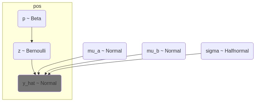
p is the probability of a bin being in compartment A, z is the latent state variable indicating whether a bin is A or B, and mu_a and mu_b are the expected means for A and B compartments, respectively. The model assumes that the E1 values are normally distributed around these means with a shared standard deviation sigma.
Let’s overwrite the model with an alternative that does not try to infer the actual state (Bernoulli part), but only draws the mean value from a Beta dist. Then, the model draw the E1 values from a mixture of mu_a and mu_b with the weights given by the probabiliy w (w and 1-w). This could be more accurate, and also it will be much faster to sample from, as we do not need to sample the latent variable z_i for each bin which is using a really slow BinaryMetropolisHastings sampler.
with pm.Model(coords={"pos": df.index.values}) as model:

    # mu_a = pm.Normal("mu_a", 0.5, 0.3)
    # mu_b = pm.Normal("mu_b", -0.5, 0.3)
    # sigma = pm.HalfNormal("sigma", 0.3)
    # New: Make ordered parameters for mu_a and mu_b in stead
    mu = pm.Normal("mu", mu=[-0.5, 0.5], sigma=0.3,
        transform=pm.distributions.transforms.ordered, # IMPORTANT
        shape=2,
        )
    sigma = pm.HalfNormal("sigma", 0.3, shape=2)

    w = pm.Beta("w", 1, 1)

    # components = pm.Normal.dist(mu = pm.math.stack([mu_a, mu_b]), sigma = sigma, shape=(2,))
    # New: Use the ordered mu parameters (cleaner code as well)
    components = pm.StudentT.dist(nu=10, mu=mu, sigma=sigma, shape=2)

    # Likelihood estimate
    y_lik = pm.Mixture("y_lik", w=[w,1-w], comp_dists=components, observed=df.e1.values)
Right, let’s rewrite it again, so that the model uses a switch again, but this time based on the latent probability og being in A.
coords = {"bins": df.index.values,
          "pos": df.start.values}

with pm.Model(coords=coords) as model_inactive:
    # Let the model be aware of the data
    ## Cannot be done with missing values or masked arrays
    #e1 = pm.Data("e1", df.e1.dropna().values, dims="bins")

    # Two means for A and B compartments
    mu_a = pm.Normal("mu_a", 0.5, 0.3)
    mu_b = pm.Normal("mu_b", -0.5, 0.3)

    # Standard deviation for the noise (only positive values HalfStudent)
    sigma = pm.HalfNormal("sigma", 0.3)

    # Latent state for each bin: 1 = A, 0 = B
    p = pm.Beta("p", 2, 2, dims="bins")

    # per-bin expected mean
    mu = pm.math.switch(p > 0.5, mu_a, mu_b)

    # Likelihood estimate
    y_lik = pm.Normal("y_lik", mu=mu, sigma=sigma, observed=df.e1.values, dims="bins")
Model graphs
# Visualize
model_graph = pm.model_to_graphviz(model)
#model_graph

model.to_graphviz()
Test the priors
with model:
    # Sample from the prior
    trace = pm.sample_prior_predictive(samples=1000)

trace
Sampling: [mu, sigma, w, y_lik]arviz.InferenceData
-
<xarray.Dataset> Size: 48kB Dimensions: (chain: 1, draw: 1000, mu_dim_0: 2, sigma_dim_0: 2) Coordinates: * chain (chain) int64 8B 0 * draw (draw) int64 8kB 0 1 2 3 4 5 6 ... 993 994 995 996 997 998 999 * mu_dim_0 (mu_dim_0) int64 16B 0 1 * sigma_dim_0 (sigma_dim_0) int64 16B 0 1 Data variables: mu (chain, draw, mu_dim_0) float64 16kB -0.8359 0.3563 ... 0.4222 w (chain, draw) float64 8kB 0.9586 0.4445 ... 0.7499 0.4273 sigma (chain, draw, sigma_dim_0) float64 16kB 0.3965 ... 0.06899 Attributes: created_at: 2025-07-17T20:04:04.066581+00:00 arviz_version: 0.21.0 inference_library: pymc inference_library_version: 5.22.0 -
<xarray.Dataset> Size: 12MB Dimensions: (chain: 1, draw: 1000, y_lik_dim_0: 1438) Coordinates: * chain (chain) int64 8B 0 * draw (draw) int64 8kB 0 1 2 3 4 5 6 ... 993 994 995 996 997 998 999 * y_lik_dim_0 (y_lik_dim_0) int64 12kB 0 1 2 3 4 ... 1433 1434 1435 1436 1437 Data variables: y_lik (chain, draw, y_lik_dim_0) float64 12MB -0.4438 ... -0.9239 Attributes: created_at: 2025-07-17T20:04:04.071089+00:00 arviz_version: 0.21.0 inference_library: pymc inference_library_version: 5.22.0 -
<xarray.Dataset> Size: 23kB
Dimensions:      (y_lik_dim_0: 1438)
Coordinates:
  * y_lik_dim_0  (y_lik_dim_0) int64 12kB 0 1 2 3 4 ... 1433 1434 1435 1436 1437
Data variables:
    y_lik        (y_lik_dim_0) float64 12kB 0.3417 0.3356 ... -0.4138 0.01386
Attributes:
    created_at:                 2025-07-17T20:04:04.072582+00:00
    arviz_version:              0.21.0
    inference_library:          pymc
    inference_library_version:  5.22.0
prior_predictive_e1 = az.extract(trace, group="prior_predictive", var_names=["y_lik"])

print(f"""
y_lik (min, max, std): {prior_predictive_e1.values.min(), prior_predictive_e1.values.max(), prior_predictive_e1.values.std()}
""")

#y_lik_norm (min, max, std): {prior_predictive_e1.y_lik_norm.values.min(), prior_predictive_e1.y_lik_norm.values.max(), prior_predictive_e1.y_lik_norm.values.std()}
y_lik (min, max, std): (np.float64(-6.262508919078938), np.float64(6.799305017469241), np.float64(0.6678983101948808))
e1_obs = df['e1'].dropna().values

az.plot_dist(
    e1_obs,
    kind="hist",
    color="C1",
    hist_kwargs={"alpha": 0.6,  "bins": 25},
    label="observed"
)


prior_pred_obs = trace.prior_predictive["y_lik"].stack(sample=("chain", "draw")).values
prior_pred_obs = prior_pred_obs[prior_pred_obs > e1_obs.min()]  # Constrain the range to observed values
prior_pred_obs = prior_pred_obs[prior_pred_obs < e1_obs.max()]  # Constrain the range to observed values

az.plot_dist(
    prior_pred_obs,
    kind="hist",
    hist_kwargs={"alpha": 0.6, "bins":25},
    label="simulated",
)
plt.xticks(rotation=90);
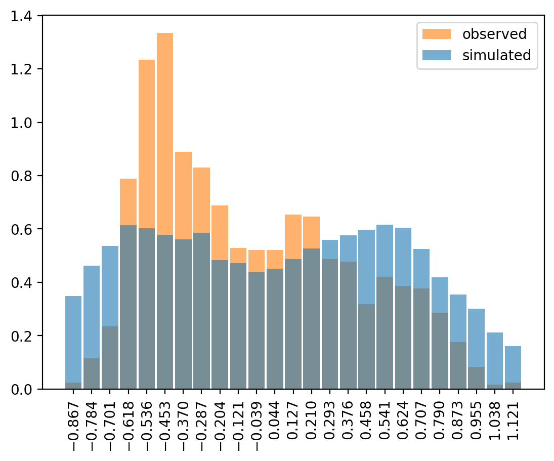
This was quite involved to get to plot, as the prior predictions take values between -Inf and Inf. It could mean that the priors are not super robust to the random variables defining the StudentT draws from y_lik: If the nu or sigma draws are too small, the T-dist could become numerically unstable and produce Inf values.
With y_lik adhering to a Normal distribution, there are no infinites, and the range is more narrow. That must mean something to the predicitions as well, but I’m not quite sure about the effect.
Posterior sampling
Here, we both create a trace (by sampling) and then sample from the predictive posterior.
with model:
    # Sample from the posterior
    trace = pm.sample(2000, tune=2000, cores=4, chains=4, target_accept=0.9,
                    #   step = [
                    #       pm.NUTS([mu_a, mu_b, sigma, p], target_accept=0.9),
                    #       pm.BinaryGibbsMetropolis([z], transit_p=0.8)],
                        #   nuts_sampler='nutpie'
                    )
Initializing NUTS using jitter+adapt_diag...
Multiprocess sampling (4 chains in 4 jobs)
NUTS: [mu, sigma, w]Sampling 4 chains for 2_000 tune and 2_000 draw iterations (8_000 + 8_000 draws total) took 12 seconds.
with model:
    pm.sample_posterior_predictive(trace, extend_inferencedata=True)
Sampling: [y_lik]with model:
prior_pred = pm.sample_prior_predictive(samples=1000)
trace.extend(prior_pred)Sampling: [mu, sigma, w, y_lik]with model:
pm.compute_log_likelihood(trace, extend_inferencedata=True)Evaluation
We now have some variables that are fitted and all have a posterior distribution.
Which ones are interesting? Well, the p represents the probability \(p \in [0;1]\) for a bin to be in compartment A (remember, A is 1, and B is 0). z is the actual compartment assignment \(z \in \{0, 1\}\), where \(z \sim \mathcal{Bernoulli}(p) = \mathcal{B}(1,p)\). y is the observed E1 value drawn from a Normal distribution with the fitted mu and sigma.
tracearviz.InferenceData
-
<xarray.Dataset> Size: 336kB Dimensions: (chain: 4, draw: 2000, mu_dim_0: 2, sigma_dim_0: 2) Coordinates: * chain (chain) int64 32B 0 1 2 3 * draw (draw) int64 16kB 0 1 2 3 4 5 ... 1994 1995 1996 1997 1998 1999 * mu_dim_0 (mu_dim_0) int64 16B 0 1 * sigma_dim_0 (sigma_dim_0) int64 16B 0 1 Data variables: mu (chain, draw, mu_dim_0) float64 128kB -0.4702 0.2515 ... 0.2362 sigma (chain, draw, sigma_dim_0) float64 128kB 0.1363 ... 0.343 w (chain, draw) float64 64kB 0.4639 0.441 0.3999 ... 0.445 0.4607 Attributes: created_at: 2025-07-17T20:04:24.272121+00:00 arviz_version: 0.21.0 inference_library: pymc inference_library_version: 5.22.0 sampling_time: 11.661832809448242 tuning_steps: 2000 -
<xarray.Dataset> Size: 92MB Dimensions: (chain: 4, draw: 2000, y_lik_dim_0: 1438) Coordinates: * chain (chain) int64 32B 0 1 2 3 * draw (draw) int64 16kB 0 1 2 3 4 5 ... 1994 1995 1996 1997 1998 1999 * y_lik_dim_0 (y_lik_dim_0) int64 12kB 0 1 2 3 4 ... 1433 1434 1435 1436 1437 Data variables: y_lik (chain, draw, y_lik_dim_0) float64 92MB 0.7819 ... -0.3133 Attributes: created_at: 2025-07-17T20:05:06.571911+00:00 arviz_version: 0.21.0 inference_library: pymc inference_library_version: 5.22.0 -
<xarray.Dataset> Size: 92MB Dimensions: (chain: 4, draw: 2000, y_lik_dim_0: 1438) Coordinates: * chain (chain) int64 32B 0 1 2 3 * draw (draw) int64 16kB 0 1 2 3 4 5 ... 1994 1995 1996 1997 1998 1999 * y_lik_dim_0 (y_lik_dim_0) int64 12kB 0 1 2 3 4 ... 1433 1434 1435 1436 1437 Data variables: y_lik (chain, draw, y_lik_dim_0) float64 92MB -0.5022 ... -0.6849 Attributes: created_at: 2025-07-17T20:05:13.737485+00:00 arviz_version: 0.21.0 inference_library: pymc inference_library_version: 5.22.0 -
<xarray.Dataset> Size: 992kB Dimensions: (chain: 4, draw: 2000) Coordinates: * chain (chain) int64 32B 0 1 2 3 * draw (draw) int64 16kB 0 1 2 3 4 ... 1996 1997 1998 1999 Data variables: (12/17) process_time_diff (chain, draw) float64 64kB 0.003304 ... 0.002189 largest_eigval (chain, draw) float64 64kB nan nan nan ... nan nan smallest_eigval (chain, draw) float64 64kB nan nan nan ... nan nan index_in_trajectory (chain, draw) int64 64kB 2 -4 -12 -4 -4 ... 6 1 -1 -7 energy (chain, draw) float64 64kB 704.5 702.1 ... 698.2 n_steps (chain, draw) float64 64kB 11.0 7.0 15.0 ... 15.0 7.0 ... ... step_size_bar (chain, draw) float64 64kB 0.5156 0.5156 ... 0.5254 step_size (chain, draw) float64 64kB 0.4825 0.4825 ... 0.5364 perf_counter_diff (chain, draw) float64 64kB 0.003322 ... 0.002204 reached_max_treedepth (chain, draw) bool 8kB False False ... False False energy_error (chain, draw) float64 64kB -0.08991 ... 0.02868 acceptance_rate (chain, draw) float64 64kB 0.9867 0.977 ... 0.9603 Attributes: created_at: 2025-07-17T20:04:24.291847+00:00 arviz_version: 0.21.0 inference_library: pymc inference_library_version: 5.22.0 sampling_time: 11.661832809448242 tuning_steps: 2000 -
<xarray.Dataset> Size: 48kB Dimensions: (chain: 1, draw: 1000, mu_dim_0: 2, sigma_dim_0: 2) Coordinates: * chain (chain) int64 8B 0 * draw (draw) int64 8kB 0 1 2 3 4 5 6 ... 993 994 995 996 997 998 999 * mu_dim_0 (mu_dim_0) int64 16B 0 1 * sigma_dim_0 (sigma_dim_0) int64 16B 0 1 Data variables: mu (chain, draw, mu_dim_0) float64 16kB -0.488 0.9919 ... 0.5711 w (chain, draw) float64 8kB 0.8434 0.286 0.7967 ... 0.1119 0.3174 sigma (chain, draw, sigma_dim_0) float64 16kB 0.08126 ... 0.619 Attributes: created_at: 2025-07-17T20:05:12.166162+00:00 arviz_version: 0.21.0 inference_library: pymc inference_library_version: 5.22.0 -
<xarray.Dataset> Size: 12MB Dimensions: (chain: 1, draw: 1000, y_lik_dim_0: 1438) Coordinates: * chain (chain) int64 8B 0 * draw (draw) int64 8kB 0 1 2 3 4 5 6 ... 993 994 995 996 997 998 999 * y_lik_dim_0 (y_lik_dim_0) int64 12kB 0 1 2 3 4 ... 1433 1434 1435 1436 1437 Data variables: y_lik (chain, draw, y_lik_dim_0) float64 12MB -0.4681 ... 0.1658 Attributes: created_at: 2025-07-17T20:05:12.169687+00:00 arviz_version: 0.21.0 inference_library: pymc inference_library_version: 5.22.0 -
<xarray.Dataset> Size: 23kB
Dimensions:      (y_lik_dim_0: 1438)
Coordinates:
  * y_lik_dim_0  (y_lik_dim_0) int64 12kB 0 1 2 3 4 ... 1433 1434 1435 1436 1437
Data variables:
    y_lik        (y_lik_dim_0) float64 12kB 0.3417 0.3356 ... -0.4138 0.01386
Attributes:
    created_at:                 2025-07-17T20:04:24.297491+00:00
    arviz_version:              0.21.0
    inference_library:          pymc
    inference_library_version:  5.22.0
Let’s do some stuff on the log-likelihood of the posterior. We can use arviz to generate Leave-One-Out (LOO) cross-validation
model_loo = az.loo(trace)
model_loo
Computed from 8000 posterior samples and 1438 observations log-likelihood matrix.
Estimate SE
elpd_loo -697.67 23.31
p_loo 4.73 -
------
Pareto k diagnostic values:
Count Pct.
(-Inf, 0.70] (good) 1438 100.0%
(0.70, 1] (bad) 0 0.0%
(1, Inf) (very bad) 0 0.0%az.plot_ppc(trace, num_pp_samples=500, group="prior", data_pairs={"y_lik": "y_lik"});
plt.legend(loc="upper right")
plt.ylim(0,10);
az.plot_ppc(trace, num_pp_samples=500, group="posterior");
plt.legend(loc="upper right")
plt.tight_layout()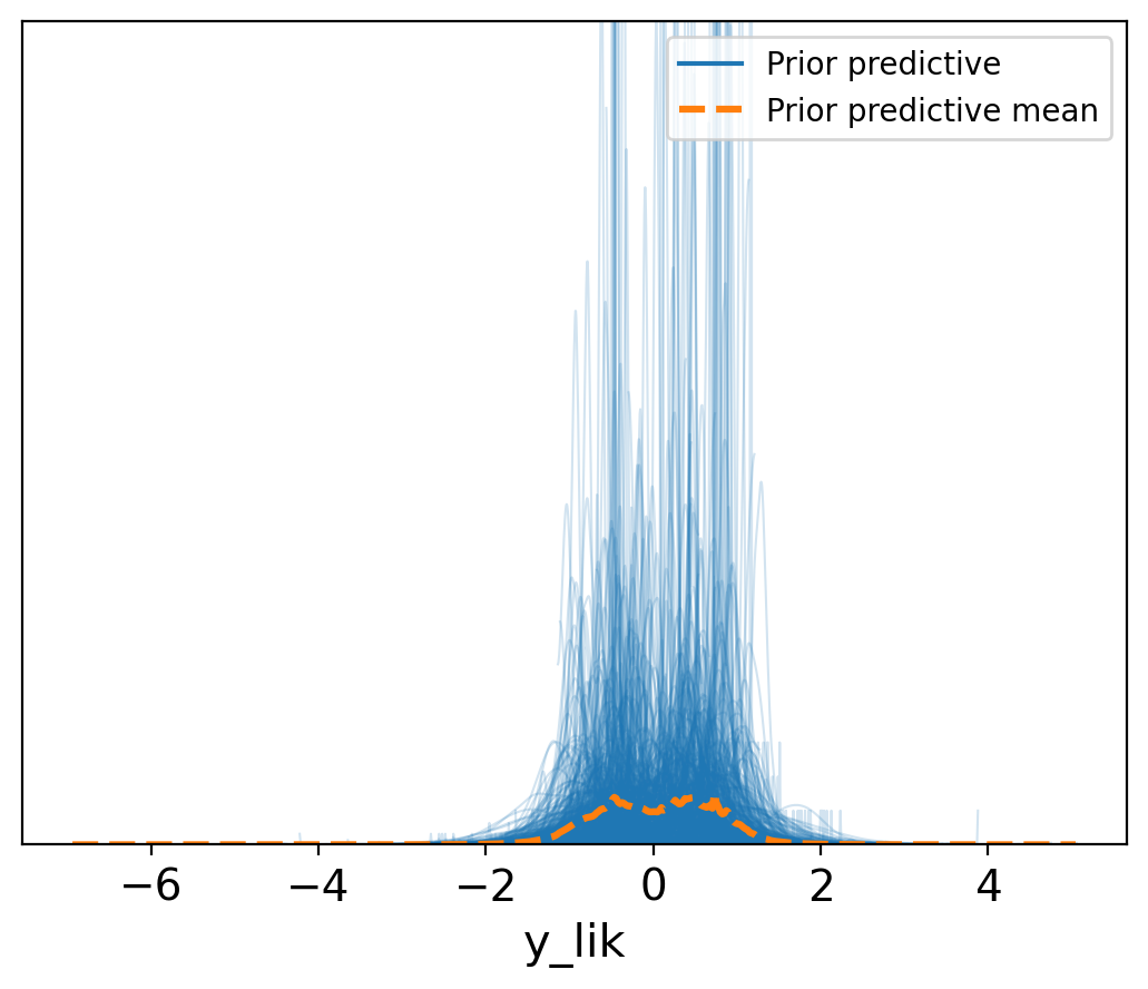
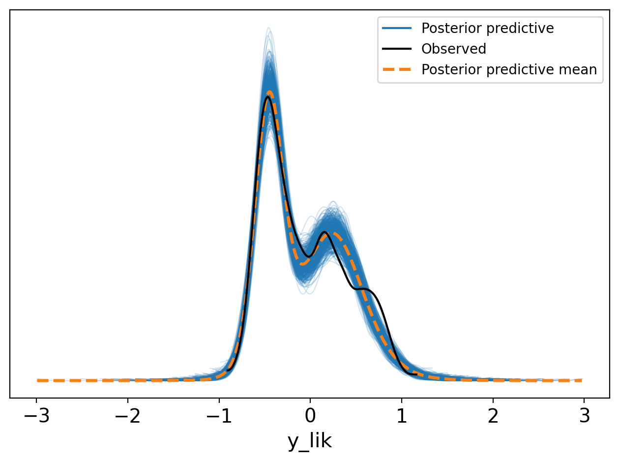
Slight deviation near 1 in the posterior predictive distribution suggests possible additional states, but the model otherwise captures the main features of the E1 distribution.
az.plot_trace(trace, var_names=["mu", 'sigma'], compact=True, backend_kwargs={'layout': 'tight'});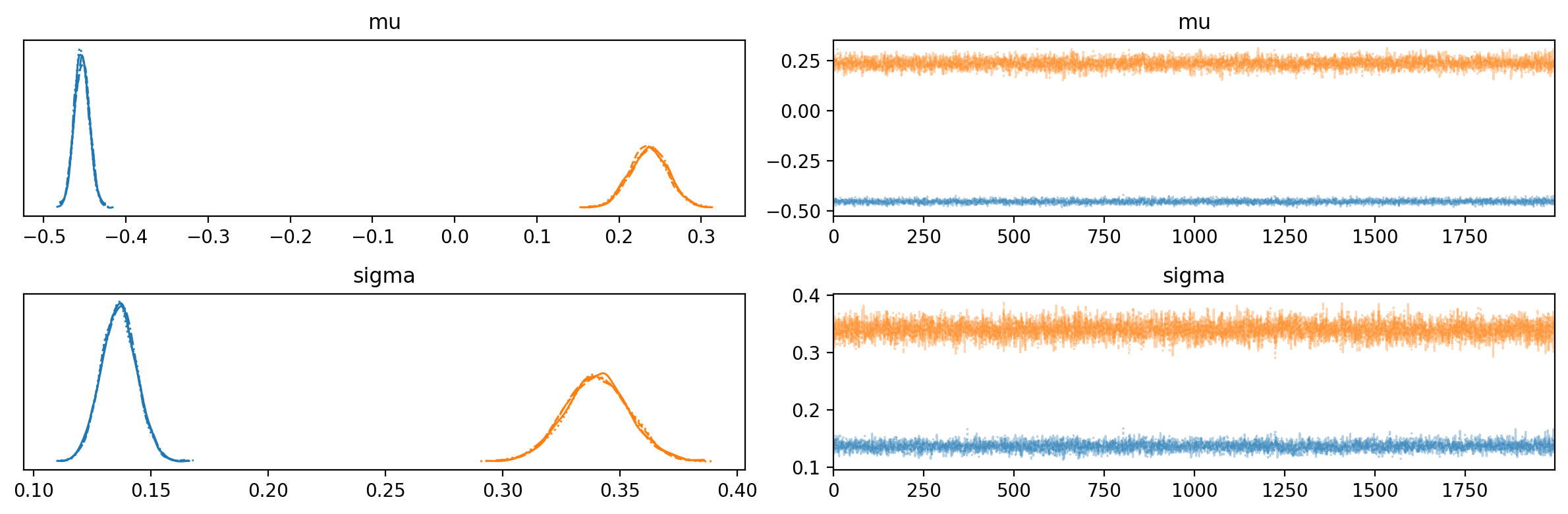
trace_ylik = az.summary(trace, var_names=['y_lik'], kind='stats', group='posterior_predictive')trace_ylik| mean | sd | hdi_3% | hdi_97% | |
|---|---|---|---|---|
| y_lik[0] | -0.075 | 0.454 | -0.696 | 0.795 |
| y_lik[1] | -0.069 | 0.453 | -0.750 | 0.748 |
| y_lik[2] | -0.075 | 0.453 | -0.750 | 0.742 |
| y_lik[3] | -0.067 | 0.459 | -0.744 | 0.750 |
| y_lik[4] | -0.074 | 0.456 | -0.746 | 0.770 |
| ... | ... | ... | ... | ... |
| y_lik[1433] | -0.067 | 0.460 | -0.737 | 0.778 |
| y_lik[1434] | -0.071 | 0.459 | -0.741 | 0.773 |
| y_lik[1435] | -0.067 | 0.458 | -0.759 | 0.750 |
| y_lik[1436] | -0.068 | 0.462 | -0.711 | 0.817 |
| y_lik[1437] | -0.070 | 0.460 | -0.741 | 0.779 |
1438 rows × 4 columns
print(pd.DataFrame({
    "mean": [trace_ylik['mean'].mean(), trace_ylik['mean'].std()],
    "sd": [trace_ylik['sd'].mean(), trace_ylik['sd'].std()]
}).set_index(pd.Index(['means', 'sds'])).round(4))

f,ax = plt.subplots(1,2, figsize=(10, 5))
ax = ax.flatten()
ax[0].set_title("Mean of y_lik estimate")
ax[0].hist(trace_ylik['mean'], bins=300, color="tab:grey", alpha=0.5)
#ax[0].set_xlim(-0.05,0.05) # zoom-in on the near-zero peak
ax[1].set_title("SD of y_lik")
ax[1].hist(trace_ylik['sd'], bins=30, color="tab:grey", alpha=0.5)
plt.tight_layout()
mean sd
means -0.0728 0.4565
sds 0.0050 0.0035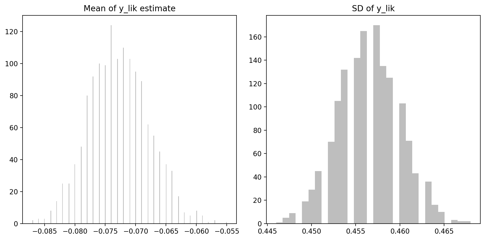
Why does it seem to contain a lot of means on zero? Let’s find out how many
(trace_ylik['mean'] == 0 ).sum()np.int64(0)Well, that was not very informative, but it looks like the peak is very close to the mean (-0.0149), and not zero (upon closer inspection).
Let’s look at the actual values from the trace.
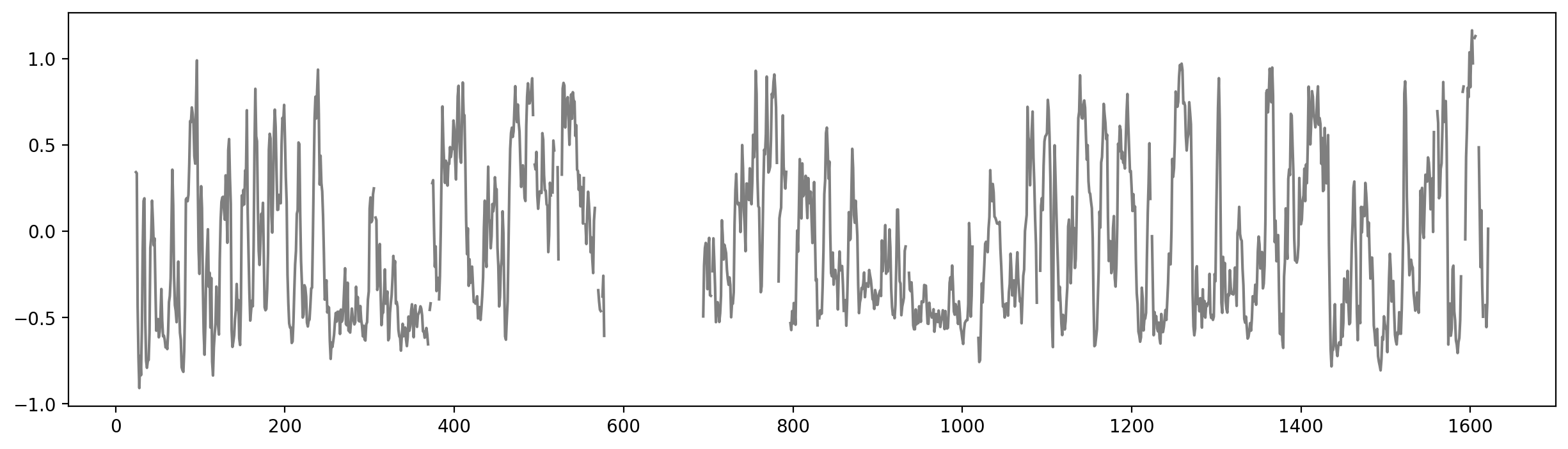
f,ax = plt.subplots(figsize=(12,4))
ax.plot(df['start'], trace_ylik['mean'], lw=0.3, label="prediction confidence")
ax.fill_between(df['start'], trace_ylik['hdi_97%'], trace_ylik['hdi_3%'], color="tab:grey", alpha=0.3, label="95% HDI")
plt.tight_layout()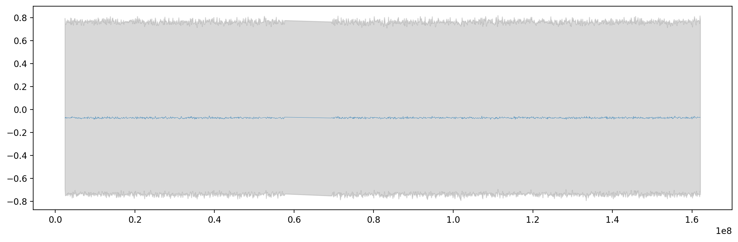
That looks promising, but we have to look at the predictive samples. Let’s look at the posterior predictive samples to see how well the model fits the data.
trace.posterior_predictive.stack(sample=("chain", "draw"))<xarray.Dataset> Size: 92MB
Dimensions: (y_lik_dim_0: 1438, sample: 8000)
Coordinates:
* y_lik_dim_0 (y_lik_dim_0) int64 12kB 0 1 2 3 4 ... 1433 1434 1435 1436 1437
* sample (sample) object 64kB MultiIndex
* chain (sample) int64 64kB 0 0 0 0 0 0 0 0 0 0 ... 3 3 3 3 3 3 3 3 3 3
* draw (sample) int64 64kB 0 1 2 3 4 5 ... 1995 1996 1997 1998 1999
Data variables:
y_lik (y_lik_dim_0, sample) float64 92MB 0.7819 0.7595 ... -0.3133
Attributes:
created_at: 2025-07-17T20:05:06.571911+00:00
arviz_version: 0.21.0
inference_library: pymc
inference_library_version: 5.22.0# p_B = trace.posterior["z"].mean(dim=["chain", "draw"]).values
y_ppc = trace.posterior_predictive["y_lik"]
y_ppc_flat = y_ppc.stack(sample=("chain", "draw"))
ppc_mean = y_ppc_flat.mean(dim="sample").values # mean of predictions per bin
ppc_std = y_ppc_flat.std(dim="sample").values # predictive std (uncertainty)
ppc_hdi = az.hdi(y_ppc, hdi_prob=0.95) # 95% HDI using ArviZPosterior predictive checks
How does the posterior predictive look? We can visualize the distribution of predicted E1s based on the posterior samples. Here, the mean and sd of the posterior predictive for each bin are visualized in histograms.
f,ax= plt.subplots(1,2, figsize=(10, 3))
ax[0].set_title("Posterior Predictive Mean of y_lik")
ax[0].set_ylabel("Counts")
ax[0].hist(ppc_mean, bins=40, alpha=0.7, label="Mean(y_lik)")
ax[1].set_title("Posterior Predictive Std of y_lik")
ax[1].hist(ppc_std, bins=40, alpha=0.7, label="Std(y_lik)")
plt.tight_layout()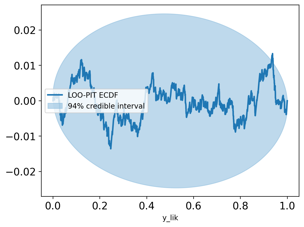
Full mixture Hmpf. That was not very promising at all. We would like the posterior predictive to match the observed E1 values, but what we get is a unimodal. Why can that be? The data is modeled as a mixture without a latent binary variable, \(z \in {0,1}\).
Latent z hard assignment Here, we do get a distribution of \(\hat{y}\) that somewhat resembles the means of the two suggested distributions for A and B compartments.
az.plot_loo_pit(trace, y_hat="y_lik", y = "y_lik", ecdf=True)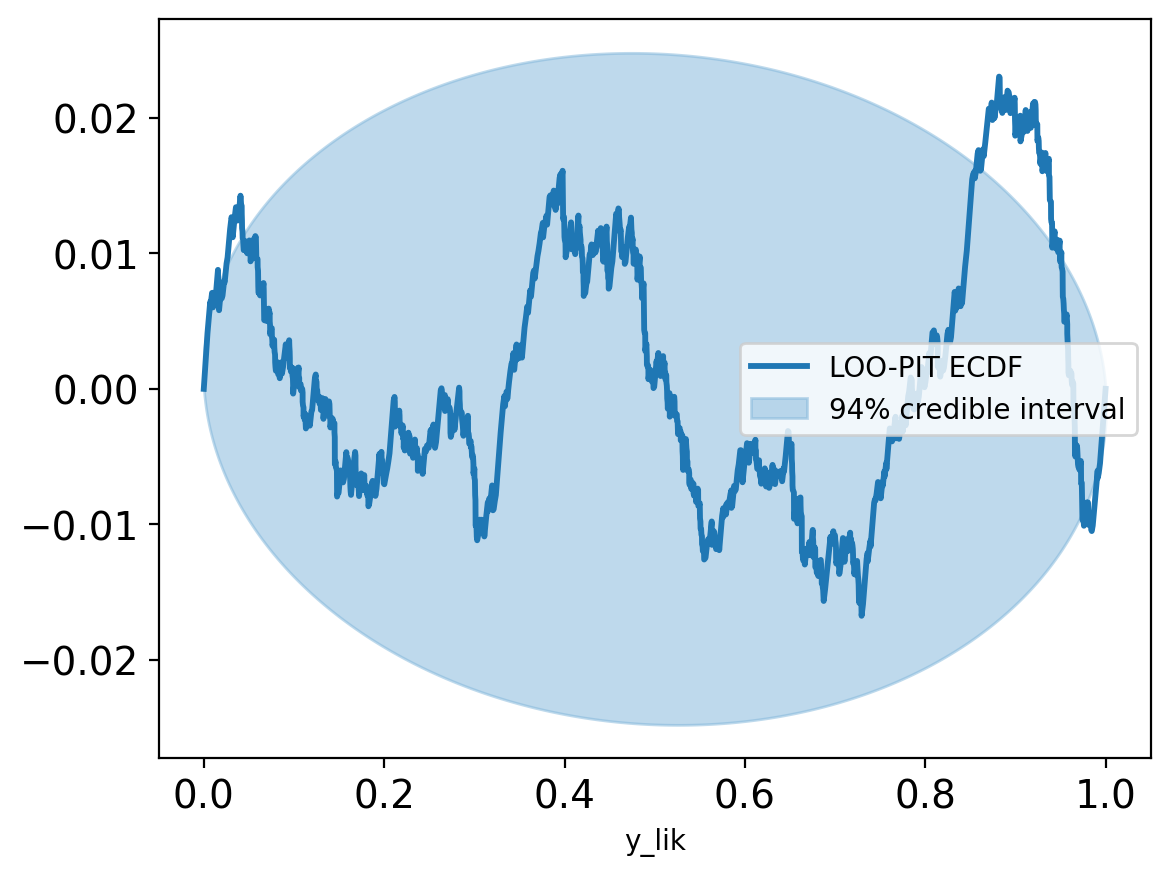
Latent z model Here, there are clear signs of overdispersion, or just something about the structure of the model that does not fit. I’m thinking the model is overdispersed as the bins are i.i.d. There is no limit on the ‘walk distance’ between the bins, so the model can easily make too large jumps between bins.
Consistency
We can also try to calculate how consistent the predicted E1 is with the observed E1. Maybe this is useful.
trace.posterior_predictive["y_lik"].mean(dim=["chain", "draw"]).valuesarray([-0.07486874, -0.06894212, -0.07457259, ..., -0.0674801 ,
-0.06846435, -0.07049419], shape=(1438,))# ppc_mean: shape (bins,)
# mean_ll: shape (bins,)
posterior_mean = trace.posterior_predictive["y_lik"].mean(dim=["chain", "draw"]).values
mean_ll = trace.log_likelihood.y_lik.mean(dim=["chain", "draw"]).values
# Plot the data as a track (stairs for niceity)
fig, ax = plt.subplots(figsize=(20, 5))
# Stairs
x_stair = np.zeros(2*y.shape[0])
y_stair = np.zeros(2*y.shape[0])
x_stair[0::2] = x
x_stair[1::2] = x + resolution
y_stair[0::2] = y
y_stair[1::2] = y
ax.fill_between(x_stair, y_stair, where=(y_stair<0), color="tab:blue", alpha=0.5, ec='None')
ax.fill_between(x_stair, y_stair, where=(y_stair>0), color="tab:red", alpha=0.5, ec='None')
# plot the y_ppc_flat mean
post_mean_stairs = np.zeros(2*y.shape[0])
post_mean_stairs[0::2] = posterior_mean
post_mean_stairs[1::2] = posterior_mean
ax.plot(x_stair, post_mean_stairs, lw=1, label="Posterior Predictive Mean", color="tab:orange")
# Plot the point-wise log-likelihood
ll_stair = np.zeros(2*mean_ll.shape[0])
ll_stair[0::2] = mean_ll
ll_stair[1::2] = mean_ll
ax.plot(x_stair, ll_stair, lw=1, label="Binwise Log-Likelihood", color="tab:green")
ax.set_xlim(0, 57_984_683)
ticks = np.arange(0, 57_984_683, step=5_000_000)
ax.set_xticks(ticks)
ax.set_xticklabels((ticks / 1e6).astype(int), rotation=45)
ax.set_xlabel("Genomic Position (Mbp)")
ax.set_ylabel("E1")
ax.set_title("E1")
ax.legend(loc="best");--------------------------------------------------------------------------- ValueError Traceback (most recent call last) Cell In[32], line 24 22 # plot the y_ppc_flat mean 23 post_mean_stairs = np.zeros(2*y.shape[0]) ---> 24 post_mean_stairs[0::2] = posterior_mean 25 post_mean_stairs[1::2] = posterior_mean 26 ax.plot(x_stair, post_mean_stairs, lw=1, label="Posterior Predictive Mean", color="tab:orange") ValueError: could not broadcast input array from shape (1438,) into shape (1623,)
bins = np.arange(len(y))

plt.figure(figsize=(15, 4))

# Observed data
plt.plot(bins, y, label="Observed E1", color="black", alpha=0.5)

# Posterior predictive mean
plt.plot(bins, ppc_mean, label="Posterior Mean", color="tab:red")

# Credible interval shading
plt.fill_between(
    bins,
    ppc_hdi.y_lik.sel(hdi='lower').values,
    ppc_hdi.y_lik.sel(hdi='higher').values,
    color="tab:red",
    alpha=0.3,
    label="95% Credible Interval"
)

plt.xlabel("Genomic bin")
plt.ylabel("E1 value")
plt.title("Posterior Predictive Mean with 95% CI")
plt.legend()
plt.tight_layout()
plt.show()
--------------------------------------------------------------------------- ValueError Traceback (most recent call last) Cell In[33], line 9 6 plt.plot(bins, y, label="Observed E1", color="black", alpha=0.5) 8 # Posterior predictive mean ----> 9 plt.plot(bins, ppc_mean, label="Posterior Mean", color="tab:red") 11 # Credible interval shading 12 plt.fill_between( 13 bins, 14 ppc_hdi.y_lik.sel(hdi='lower').values, (...) 18 label="95% Credible Interval" 19 ) File ~/miniconda3/envs/pymc/lib/python3.13/site-packages/matplotlib/pyplot.py:3838, in plot(scalex, scaley, data, *args, **kwargs) 3830 @_copy_docstring_and_deprecators(Axes.plot) 3831 def plot( 3832 *args: float | ArrayLike | str, (...) 3836 **kwargs, 3837 ) -> list[Line2D]: -> 3838 return gca().plot( 3839 *args, 3840 scalex=scalex, 3841 scaley=scaley, 3842 **({"data": data} if data is not None else {}), 3843 **kwargs, 3844 ) File ~/miniconda3/envs/pymc/lib/python3.13/site-packages/matplotlib/axes/_axes.py:1777, in Axes.plot(self, scalex, scaley, data, *args, **kwargs) 1534 """ 1535 Plot y versus x as lines and/or markers. 1536 (...) 1774 (``'green'``) or hex strings (``'#008000'``). 1775 """ 1776 kwargs = cbook.normalize_kwargs(kwargs, mlines.Line2D) -> 1777 lines = [*self._get_lines(self, *args, data=data, **kwargs)] 1778 for line in lines: 1779 self.add_line(line) File ~/miniconda3/envs/pymc/lib/python3.13/site-packages/matplotlib/axes/_base.py:297, in _process_plot_var_args.__call__(self, axes, data, return_kwargs, *args, **kwargs) 295 this += args[0], 296 args = args[1:] --> 297 yield from self._plot_args( 298 axes, this, kwargs, ambiguous_fmt_datakey=ambiguous_fmt_datakey, 299 return_kwargs=return_kwargs 300 ) File ~/miniconda3/envs/pymc/lib/python3.13/site-packages/matplotlib/axes/_base.py:494, in _process_plot_var_args._plot_args(self, axes, tup, kwargs, return_kwargs, ambiguous_fmt_datakey) 491 axes.yaxis.update_units(y) 493 if x.shape[0] != y.shape[0]: --> 494 raise ValueError(f"x and y must have same first dimension, but " 495 f"have shapes {x.shape} and {y.shape}") 496 if x.ndim > 2 or y.ndim > 2: 497 raise ValueError(f"x and y can be no greater than 2D, but have " 498 f"shapes {x.shape} and {y.shape}") ValueError: x and y must have same first dimension, but have shapes (1623,) and (1438,)
Next up: Introducing dependency between bins
In the next notebook, we will implement a Gaussian Random Walk (GRW) model to introduce spatial dependency between bins. We will investigate how it affects smoothing and uncertainty in compartment assignment.
We will update the model to
\[\begin{aligned} p_t &\sim \mathcal{N}(p_{t-1}, \sigma^2_{t-1}) \\ z_t &\sim \text{Bernoulli}(p_t) \\ \\ \mu_{z_t} &= z_t \cdot \mu_A + (1 - z_t) \cdot \mu_B \\ y_t &\sim \mathcal{N}(\mu_{z_t}, \sigma^2) \end{aligned}\]