Compartments Analysis w. recommended parameters

Analysis of Chromatin Compartments using the Open2C Ecosystem and their recommended paramters

NB: This notebook is a duplicate of 03_compartments but on new coolers with recommended parameters for pairtools parse and cooler cload.

Working with coolers

In this notebook, we use files generated by workflow.py that, in short, does the following:

1. Download the data from the source
2. Index the reference genome with bwa index and samtools faidx
3. Align the reads to the reference genome with bwa mem
4. Pair and sort the reads to .pairs files with pairtools parse | pairtools sort
5. Deduplicate the pairs with pairtools dedup
6. Convert the .pairs to cooler files with pairtools select $filter | cooler cload pairs
   • filter="mapq1>=30 and mapq2 >= 30"

We will:

1. Load the cooler files
2. Merge the coolers from the same BioSample ID –> Create ‘replicates’
3. Zoomify the merged cooler files (coarsen) to create a multicooler (.mcool) file
4. Balance the matrices (use commandline cooler balance)
5. Calculate E1 compartments with cooltools compute_cis_eig

Overview

Data (Accessions)

To get an overview of the data accessions used in this analysis, we will first summarize the SRA-runtable.tsv that contains the accession numbers and some metadata for each sample (Table 17.1).

Table 7.1: The most relevant columns of the SRA-runtable.tsv file

	source_name	BioSample	Run	GB	Bases	Reads
16	fibroblast	SAMN08375237	SRR6502335	29.771059	73,201,141,800	244,003,806
17	fibroblast	SAMN08375237	SRR6502336	22.755361	65,119,970,100	217,066,567
18	fibroblast	SAMN08375236	SRR6502337	21.434722	52,769,196,300	175,897,321
19	fibroblast	SAMN08375236	SRR6502338	21.420030	52,378,949,100	174,596,497
20	fibroblast	SAMN08375236	SRR6502339	10.207410	28,885,941,600	96,286,472
9	fibroblast	SAMN08375237	SRR7349189	52.729173	139,604,854,200	465,349,514
10	fibroblast	SAMN08375236	SRR7349190	53.085520	142,008,353,400	473,361,178
21	pachytene spermatocyte	SAMN08375234	SRR6502342	60.258880	150,370,993,500	501,236,645
22	pachytene spermatocyte	SAMN08375234	SRR6502344	27.146048	65,697,684,300	218,992,281
23	pachytene spermatocyte	SAMN08375234	SRR6502345	26.202707	63,490,538,700	211,635,129
0	pachytene spermatocyte	SAMN09427370	SRR7345458	55.970557	153,281,577,900	510,938,593
1	pachytene spermatocyte	SAMN09427370	SRR7345459	53.982492	144,993,841,200	483,312,804
11	pachytene spermatocyte	SAMN08375235	SRR7349191	51.274476	137,821,979,100	459,406,597
24	round spermatid	SAMN08375232	SRR6502351	20.924497	55,095,075,300	183,650,251
25	round spermatid	SAMN08375232	SRR6502352	41.133960	115,578,475,800	385,261,586
26	round spermatid	SAMN08375232	SRR6502353	36.444117	96,195,161,400	320,650,538
2	round spermatid	SAMN09427369	SRR7345460	38.244654	104,105,827,200	347,019,424
3	round spermatid	SAMN09427369	SRR7345461	53.996261	144,532,309,500	481,774,365
12	round spermatid	SAMN08375232	SRR7349192	52.384556	140,431,608,000	468,105,360
29	sperm	SAMN08375229	SRR6502360	26.653940	64,752,370,800	215,841,236
30	sperm	SAMN08375228	SRR6502362	23.973440	58,369,232,700	194,564,109
13	sperm	SAMN08375229	SRR7349193	52.806276	141,148,572,300	470,495,241
14	sperm	SAMN08375229	SRR7349195	22.444378	60,523,788,600	201,745,962
15	sperm	SAMN08375229	SRR7349196	38.253606	104,119,671,000	347,065,570
27	spermatogonia	SAMN08375231	SRR6502356	22.845286	58,909,579,800	196,365,266
28	spermatogonia	SAMN08375231	SRR6502357	17.947471	46,888,332,900	156,294,443
4	spermatogonia	SAMN09427379	SRR7345462	18.686342	52,032,780,000	173,442,600
5	spermatogonia	SAMN09427379	SRR7345463	29.956561	82,384,836,000	274,616,120
6	spermatogonia	SAMN09427379	SRR7345464	39.145759	105,153,716,100	350,512,387
7	spermatogonia	SAMN09427378	SRR7345465	35.816184	96,048,594,600	320,161,982
8	spermatogonia	SAMN09427378	SRR7345467	28.396816	77,248,140,900	257,493,803

Table 7.2: Summary of the data accessions used in this analysis

	source_name	GB	Bases	Reads
0	fibroblast	211.403275	553,968,406,500	1,846,561,355
1	pachytene spermatocyte	274.835160	715,656,614,700	2,385,522,049
2	round spermatid	243.128044	655,938,457,200	2,186,461,524
3	sperm	164.131640	428,913,635,400	1,429,712,118
4	spermatogonia	192.794420	518,665,980,300	1,728,886,601

Folder structure

For ease of mind, here is the folder structure of the project. ../steps/bwa/recPE/ is the base directory artificially defined in the master_workflow.py. It ccould be any other directory inside steps. It is defined relative to the workflow.py file (inside the worklow with os.path.dirname(__file__)), and converted to an absolute path by python.

../steps/bwa/recPE
├── cool
│   ├── fibroblast
│   ├── pachytene_spermatocyte
│   ├── round_spermatid
│   ├── sperm
│   └── spermatogonia
└── pairs
    ├── fibroblast
    ├── pachytene_spermatocyte
    ├── round_spermatid
    ├── sperm
    └── spermatogonia

12 directories

Figure 7.1

FullMerge (pool all from each source_name)

We will use cooler merge to merge all samples in each sub-folder (cell type) to just one interaction matrix for each cell type. The reason for that is that we choose to trust (Wang et al. 2019) when they say that compartments are highly reproducible between replicates, and by merging all replicates, we will have a more robust signal.

Thus, we will merge all samples from the same source_name into a single cooler file. The coolers are produced to only contain the real chromosomes (1-22, X, Y), and not the mitochondrial DNA or the unplaced contigs (~2,900), as they would not bring any information to the analysis.

Overview of this section:

• Locate the coolers (glob –> dictionary)
• Merge the coolers (cooler.merge_coolers)
• Zoomify the merged cooler (cooler.zoomify_cooler) to resolutions: 10kb, 50kb, 100kb, 500kb.
• Balance the matrices (!cooler balance) (use the CLI, as it is more easily parallelized)

Create cooler dictionary (glob)

First, we will create a dictionary with the paths to the coolers for each sample. We use glob.glob to fetch all the coolers in each sub-folder that remain after filtering and (automatic) quality control (those are the ones with nodups in their names).

import glob
import os.path as op
from pprint import pprint as pp
import pandas as pd

# Get the list of cell type dirs
base_dir = '../steps/bwa/recPE/cool'
folders = glob.glob(op.join(base_dir, '*'))

files_dict = {f:glob.glob(f"{f}/*.nodups.*") for f in folders}
cooler_dict = {op.basename(k): [op.basename(f) for f in v] for k,v in files_dict.items()}
#pp(cooler_dict)
df = pd.DataFrame.from_dict(cooler_dict, orient='index').T.fillna('-')
df[['fibroblast', 'spermatogonia', 'pachytene_spermatocyte', 'round_spermatid', 'sperm']].map(lambda x: x.split('.')[0])

Table 7.3: Dictionary of coolers for each cell type

	fibroblast	spermatogonia	pachytene_spermatocyte	round_spermatid	sperm
0	SRR6502338	SRR6502356	SRR7345459	SRR7345461	SRR7349195
1	SRR7349189	SRR7345467	SRR6502344	SRR6502351	SRR6502360
2	SRR6502335	SRR6502357	SRR6502342	SRR7345460	SRR7349193
3	SRR6502339	SRR7345463	SRR7345458	SRR6502352	SRR7349196
4	SRR7349190	SRR7345465	SRR7349191	SRR7349192	SRR6502362
5	SRR6502337	SRR7345462	SRR6502345	SRR6502353	-
6	SRR6502336	SRR7345464	-	-	-

Merge coolers

The coolers are merged by summing each bin in the matrices, meaning we can only merge matrices with same dimensions. We iterate through the dictionary and merge the coolers with cooler merge. The mergebuf parameter should be adjusted if you don’t have 32G memory. Default: mergebuf = 20000000. Below, we also check if the output file already exists. If it does, we skip the merge.

# NB adjust `mergebuf` if you don't have 32G of RAM

import cooler

for folder,cooler_list in cooler_dict.items():
    in_uris = [op.join(base_dir, folder, file) for file in cooler_list]
    out_uri = op.join(base_dir, folder, f'{folder}.fullmerge.cool')

    if op.exists(out_uri):
        print(f"Skipping {out_uri}: exists...")
        continue

    print(f"Creating {out_uri} by \nMerging {len(cooler_list)} coolers into one:", end=" ")
    print("\t",[file.split('.')[0] for file in cooler_list])
    cooler.merge_coolers(output_uri=out_uri,
                         input_uris=in_uris,
                         mergebuf=int(5e7),
                         )
    print("... Done!")

Creating ../steps/bwa/recPE/cool/pachytene_spermatocyte/pachytene_spermatocyte.fullmerge.cool by 
Merging 6 coolers into one:      ['SRR7345459', 'SRR6502344', 'SRR6502342', 'SRR7345458', 'SRR7349191', 'SRR6502345']

/home/sojern/miniconda3/envs/hic/lib/python3.12/site-packages/dask/dataframe/_pyarrow_compat.py:15: FutureWarning: Minimal version of pyarrow will soon be increased to 14.0.1. You are using 13.0.0. Please consider upgrading.
  warnings.warn(

... Done!
Creating ../steps/bwa/recPE/cool/spermatogonia/spermatogonia.fullmerge.cool by 
Merging 7 coolers into one:      ['SRR6502356', 'SRR7345467', 'SRR6502357', 'SRR7345463', 'SRR7345465', 'SRR7345462', 'SRR7345464']
... Done!
Creating ../steps/bwa/recPE/cool/fibroblast/fibroblast.fullmerge.cool by 
Merging 7 coolers into one:      ['SRR6502338', 'SRR7349189', 'SRR6502335', 'SRR6502339', 'SRR7349190', 'SRR6502337', 'SRR6502336']
... Done!
Creating ../steps/bwa/recPE/cool/round_spermatid/round_spermatid.fullmerge.cool by 
Merging 6 coolers into one:      ['SRR7345461', 'SRR6502351', 'SRR7345460', 'SRR6502352', 'SRR7349192', 'SRR6502353']
... Done!
Creating ../steps/bwa/recPE/cool/sperm/sperm.fullmerge.cool by 
Merging 5 coolers into one:      ['SRR7349195', 'SRR6502360', 'SRR7349193', 'SRR7349196', 'SRR6502362']
... Done!

Zoomify the merged cooler files

After merging the coolers, we will zoomify them to resolutions: 10kb, 50kb, 100kb, 500kb. It will recursively create the zoom levels for the cooler file from the ‘base’ resolution (in our case 10kb bins) to the ‘max’ resolution (in our case 500kb bins), and save all zoom levels in a multi-resolution cooler (.mcool) file. The resolutions are stored under the resolutions key in the cooler file (e.g. cell_type.mcool::/resolutions/10000).

Here, we also check if the output file already exists. If it does, we skip the zoomify. Again, can tailor the chunksize (pixels loaded per process) parameter according to memory availability. I found that the command stalled completely (without quitting) when the memory allocation was not sufficient, as I started out with 32 cores and 32G of RAM. I did not test what was more time-efficient; increasing number of processes or chunksize. After all, it didn’t take long to run anyways.

Finally, I list the resolutions in the mcool file.

# NB 8 cores and 32G of RAM was used

import glob
import cooler
import os.path as op

base_dir = '../steps/bwa/recPE/cool'
merged_coolers = glob.glob(op.join(base_dir, '*/*.fullmerge.cool'))


for clr in merged_coolers:
    out_uri = clr.replace('.fullmerge.cool', '.mcool')
    if op.exists(out_uri):
        print(f"Skipping {out_uri}: exists...")
        continue

    print(f"Zoomifying cooler: \n\t   {clr}\n\t-> {out_uri}", end="")
    
    cooler.zoomify_cooler(base_uris = clr,
                          outfile = out_uri,
                          resolutions = [10000,50000,100000,500000],
                          chunksize = 10000000,
                          nproc = 8)
    print(" --> done")

Zoomifying cooler: 
       ../steps/bwa/recPE/cool/pachytene_spermatocyte/pachytene_spermatocyte.fullmerge.cool
    -> ../steps/bwa/recPE/cool/pachytene_spermatocyte/pachytene_spermatocyte.mcool

/home/sojern/miniconda3/envs/hic/lib/python3.12/site-packages/dask/dataframe/_pyarrow_compat.py:15: FutureWarning: Minimal version of pyarrow will soon be increased to 14.0.1. You are using 13.0.0. Please consider upgrading.
  warnings.warn(

 --> done
Zoomifying cooler: 
       ../steps/bwa/recPE/cool/spermatogonia/spermatogonia.fullmerge.cool
    -> ../steps/bwa/recPE/cool/spermatogonia/spermatogonia.mcool --> done
Zoomifying cooler: 
       ../steps/bwa/recPE/cool/fibroblast/fibroblast.fullmerge.cool
    -> ../steps/bwa/recPE/cool/fibroblast/fibroblast.mcool --> done
Zoomifying cooler: 
       ../steps/bwa/recPE/cool/round_spermatid/round_spermatid.fullmerge.cool
    -> ../steps/bwa/recPE/cool/round_spermatid/round_spermatid.mcool --> done
Zoomifying cooler: 
       ../steps/bwa/recPE/cool/sperm/sperm.fullmerge.cool
    -> ../steps/bwa/recPE/cool/sperm/sperm.mcool --> done

import glob
import cooler
mcools = glob.glob("../steps/bwa/recPE/cool/*/*.mcool")

for mcool in mcools:
    print(f"{mcool}:")
    print(cooler.fileops.list_coolers(mcool))
    print()

../steps/bwa/recPE/cool/pachytene_spermatocyte/pachytene_spermatocyte.mcool:
['/resolutions/10000', '/resolutions/50000', '/resolutions/100000', '/resolutions/500000']

../steps/bwa/recPE/cool/spermatogonia/spermatogonia.mcool:
['/resolutions/10000', '/resolutions/50000', '/resolutions/100000', '/resolutions/500000']

../steps/bwa/recPE/cool/fibroblast/fibroblast.mcool:
['/resolutions/10000', '/resolutions/50000', '/resolutions/100000', '/resolutions/500000']

../steps/bwa/recPE/cool/round_spermatid/round_spermatid.mcool:
['/resolutions/10000', '/resolutions/50000', '/resolutions/100000', '/resolutions/500000']

../steps/bwa/recPE/cool/sperm/sperm.mcool:
['/resolutions/10000', '/resolutions/50000', '/resolutions/100000', '/resolutions/500000']

Balance the matrices

Finally, we balance the matrices using the cooler CLI. We use the cooler balance command with the default options using 32 cores, which iteratively balances the matrix (Iterative Corecction). It is first described as a method for bias correction of Hi-C matrices in (Imakaev et al. 2012), where it is paired with eigenvector decomposition (ICE). Here the eigenvector decomposition of the obtained maps is shown to provide insights into local chromatin states.

According to cooler documentation, we have to balance the matrices on each resolution, and thus it cannot be done prior to zoomifying. The argument is that the balancing weights are resolution-specific and will no longer retain its meaning when binned with other weights. Therefore, we use a nested for-loop that iterates through all the .mcools and all the resolutions in each .mcool. cooler balance will create a new column in the bins group of each cooler , weight, which can then be included or not in the downstream analysis. This means we will have access to both the balanced and the unbalanced matrix.

The default mode uses genome-wide data to calculate the weights for each bin. It would maybe be more suitable to calculate the weights for cis contacts only, and that is possible through the --cis-only flag, and that can be added to another column, so that we can compare the difference between the two methods easily. However, we will only use the default mode for now. The default options are:

• ignore-diags: 2 (ignore the diagonals (-1,0,1))
• mad-max: 5 (median absolute deviation threshold)
• min-nnz: 10 (minimum number of non-zero entries before exclusion)

Conveniently, cooler balance automatically checks if there is already a weight column, and skips the balancing if it already exists. We can overwrite with --force.

%%capture balance_out --no-stderr

import sys
import glob

mcools = glob.glob("../steps/bwa/recPE/cool/*/*.mcool")
resolutions = [10000, 50000, 100000, 500000]

for mcool in mcools:
    print(f"Balancing {mcool}:", file=sys.stderr)
    for res in resolutions:
        full_name = f"{mcool}::resolutions/{res}"
        print(f"\tresolution {res}...", end=" ", file=sys.stderr)
        # First, just default values except chunksize (will write to --name weights)
        !cooler balance -p 32 {full_name}
        print("--> 'weights' done!", file=sys.stderr)
        # With only cis-contacts, write to --name cis_weights : It takes ages, maybe not worth it or submit jobs
        # !cooler balance -p 32 --cis-only --name cis_weights {full_name}
        #print("... 'cis_weights' done!", file=sys.stderr)

Balancing ../steps/bwa/recPE/cool/pachytene_spermatocyte/pachytene_spermatocyte.mcool:
    resolution 10000... --> 'weights' done!
    resolution 50000... --> 'weights' done!
    resolution 100000... --> 'weights' done!
    resolution 500000... --> 'weights' done!
Balancing ../steps/bwa/recPE/cool/spermatogonia/spermatogonia.mcool:
    resolution 10000... --> 'weights' done!
    resolution 50000... --> 'weights' done!
    resolution 100000... --> 'weights' done!
    resolution 500000... --> 'weights' done!
Balancing ../steps/bwa/recPE/cool/fibroblast/fibroblast.mcool:
    resolution 10000... --> 'weights' done!
    resolution 50000... --> 'weights' done!
    resolution 100000... --> 'weights' done!
    resolution 500000... --> 'weights' done!
Balancing ../steps/bwa/recPE/cool/round_spermatid/round_spermatid.mcool:
    resolution 10000... --> 'weights' done!
    resolution 50000... --> 'weights' done!
    resolution 100000... --> 'weights' done!
    resolution 500000... --> 'weights' done!
Balancing ../steps/bwa/recPE/cool/sperm/sperm.mcool:
    resolution 10000... --> 'weights' done!
    resolution 50000... --> 'weights' done!
    resolution 100000... --> 'weights' done!
    resolution 500000... --> 'weights' done!

# Display the balancing stdout if you want (but it is up to 200 lines per cooler)
#balance_out()

RepMerge (pool all from each BioSample ID)

Initially, I planned to re-create the replicates that they used in the paper, but I reason that it is not necessary and might even be better to pool all the samples in stead. They state alredy that their compartments are highly repdoducible between replicates, so I choose to trust that and not bother with the replicates.

Therefore, this section was only briefly initialized, and now it is commented out.

#df.groupby(['source_name','BioSample'])['Reads'].sum()

# from pprintpp import pprint as pp

# grouped_df = df.groupby(['source_name','BioSample'])

# # Initialize an empty dictionary
# rep_dict = {}

# # Iterate over each group
# for (source_name, BioSample), group in grouped_df:
#     # Extract the 'Run' column and convert it to a list
#     run_list = group['Run'].tolist()
    
#     # Populate the nested dictionary
#     if source_name not in rep_dict:
#         rep_dict[source_name] = {}
#     rep_dict[source_name][BioSample] = run_list

# pp(rep_dict)

# for source_name, BioSample_dict in rep_dict.items():
#     print(f"source_name: {source_name}")
#     print(f"Changing working dir: {source_name}/")
#     for BioSample, run_list in BioSample_dict.items():
#         print(f"Merging samples for BioSample: {BioSample}: {run_list}")

Plotting

Set up inline backend

print({key:plt.rcParams[key] for key in notebook_rcparams.keys()})

{'font.size': 10.0, 'axes.titlesize': 'large', 'axes.labelsize': 'medium', 'xtick.labelsize': 'medium', 'ytick.labelsize': 'medium', 'figure.titlesize': 'large', 'figure.figsize': [6.4, 4.8], 'figure.labelsize': 'large'}

The following section contains the visualization of the matrices and includes the calculation of the E1 compartments and their visualization. I discuss differents methods for construction and try to get both methodologically and result-wise close to (Wang et al. 2019).

First, we will work on matrices in 500kb resolution, as documentation [maybe it was HiCExplorer??] states it is sufficient for chromosome-wide analysis and plotting. We will follow the cooltools-recommended pipeline (except that they use a 100kb cooler) for visualization and compartment calling with one example cooler (the merged fibroblast cooler at 500kb resolution).

Then, the most relevant parts will be generalized to run in a loop over all the coolers. First at 500kb resolution, then at 100kb resolution.

To accomodate the approach (barely) described in the paper, we will discuss a smoothing step to the observed/expected matrices before compartment calling, and we will apply a smoothing step to the E1 compartments and compare to the raw compartments.

Example with a single sample

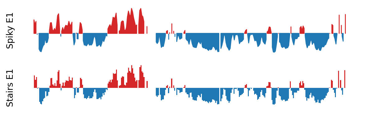
First, I will explore the visualization pipeline for a single cooler at 500kb resolution. I will modify the plot to be ‘stairs’ in stead of just a regular line plot, as it is both a more accurate representation of the data and it is more aesthetically pleasing with less spiky lines and holes.

In practice, the length of the dataframe is doubled, as it now contains an E1 value for both the start and end position for each bin in stead of only for the start. However, I first make the regular line plot to show the difference.

Imports

# import standard python libraries
import numpy as np
#import matplotlib.pyplot as plt
import pandas as pd
import os, subprocess

# Import python package for working with cooler files and tools for analysis
import cooler
import cooltools.lib.plotting
import cooltools

Load cooler

mclr = "../steps/bwa/recPE/cool/round_spermatid/round_spermatid.mcool"

clr = cooler.Cooler(f"{mclr}::resolutions/500000")

Calculate gc covariance (from the reference genome)

I will use bioframe to load the reference and calculate the GC content of each bin in the cooler file. The convention in Hi-C is to use GC content as a phasing track to orient eigenvector track to positively correlated with the GC content. In this subsection, I calculate the GC content for all chromosomes and filter afterwards to only include the ‘X’ chromosome. I will do that smarter in the next subsection.

import bioframe
import os

bins = clr.bins()[:]
rheMac10 = bioframe.load_fasta('../data/links/ucsc_ref/rheMac10.fa')
gc_cov_csv = '../steps/rheMac10_gc_cov_500kb.tsv'
if not os.path.exists(gc_cov_csv):
    print('Calculate the fraction of GC basepairs for each bin')
    gc_cov = bioframe.frac_gc(bins[['chrom', 'start', 'end']], rheMac10)
    gc_cov.to_csv(gc_cov_csv, index=False, sep='\t')
    display(gc_cov)
else: 
    print("Already exists, just read from file:")
    gc_cov = pd.read_csv(gc_cov_csv, sep='\t')
    display(gc_cov)

Already exists, just read from file:

	chrom	start	end	GC
0	chr1	0	500000	0.424508
1	chr1	500000	1000000	0.378836
2	chr1	1000000	1500000	0.388272
3	chr1	1500000	2000000	0.445226
4	chr1	2000000	2500000	0.439485
...	...	...	...	...
5715	chrY	9500000	10000000	0.399518
5716	chrY	10000000	10500000	0.396028
5717	chrY	10500000	11000000	0.395280
5718	chrY	11000000	11500000	0.382006
5719	chrY	11500000	11753682	NaN

5720 rows × 4 columns

Calculate the E1 compartments

Here, I will calculate the E1 compartments for the ‘X’ chromosome in the fibroblast cooler at 500kb resolution. I will use the cooltools package to do eigendecomposition and calculate the E1 compartments. I use the GC content (gc_cov obtained above) as a phasing track.

I will only calculate the within-chromosomes compartmentalization (cis contacts). I use cooltools.eigs_cis that decorrelate the contact-frequency by distance before performing the eigendecomposition.

I this example, I will use the simplest ‘view’ (chromosome-wide) of the chromosome to calculate the E1 values, but later I will explore how partitioning the chromosome affects the E1 values. As the GC content was calculated for all chromosomes, the eigenvectors are also calculated for the whole matrix. This will also be optimized in the next subsection, as we only ever look at the ‘X’ chromosome.

# Make the full view frame
view_df = pd.DataFrame(
    {
    'chrom': clr.chromnames,
    'start': 0,
    'end': clr.chromsizes.values,
    'name': clr.chromnames
    }
                      )
#display(view_df)

# obtain first 3 eigenvectors
cis_eigs = cooltools.eigs_cis(
                        clr,
                        gc_cov,
                        view_df=view_df,
                        n_eigs=3,
                        )

# cis_eigs[0] returns eigenvalues, here we focus on eigenvectors
eigenvector_track = cis_eigs[1][['chrom','start','end','E1']]
len(eigenvector_track)

5720

# full track
eigenvector_track

	chrom	start	end	E1
0	chr1	0	500000	NaN
1	chr1	500000	1000000	NaN
2	chr1	1000000	1500000	-0.541598
3	chr1	1500000	2000000	0.120007
4	chr1	2000000	2500000	0.377245
...	...	...	...	...
5715	chrY	9500000	10000000	NaN
5716	chrY	10000000	10500000	0.261198
5717	chrY	10500000	11000000	0.834102
5718	chrY	11000000	11500000	NaN
5719	chrY	11500000	11753682	NaN

5720 rows × 4 columns

As I have made myself a detour and calculated the eigenvectors for all chromosomes, I will now filter the eigenvector track to only include the ‘X’ chromosome. Then, I will (in the name of explicitness) construct an array of all the indices where the E1 values change sign. This is the simplest way to save the coordinates of the compartment boundaries. It can later on be saved to .csv or whatever for comparison between different samples. Also, it will be simplified in the next subsection.

# subset the chrX   
eigenvector_track_chrX = eigenvector_track.loc[eigenvector_track['chrom'] == 'chrX']
nbins = len(eigenvector_track_chrX)
eigenvector_track_chrX
e1X_values = eigenvector_track_chrX['E1'].values

# Where does the E1 change sign
np.where(np.diff( (cis_eigs[1][cis_eigs[1]['chrom']=='chrX']['E1']>0).astype(int)))[0]

array([  1,   4,   5,   6,  16,  27,  28,  39,  42,  43,  45,  49,  73,
        83,  84, 102, 103, 109, 111, 112, 130, 132, 133, 134, 135, 136,
       137, 138, 147, 149, 206, 209, 228, 233, 239, 240, 251, 252, 260,
       265, 289, 290, 291, 293, 298, 299, 300, 301, 304, 305])

Plot E1 and matrix

Finally, I will plot the matrix, the GC content, and the E1 compartments for the ‘X’ chromosome in the fibroblast cooler at 500kb resolution. I will use the cooltools package to plot the matrix and the compartments. I will use the matplotlib package to plot the GC content.

I will plot the matrix as a heatmap, the GC content as a line plot, and the E1 compartments as a line plot. I will also plot the compartment boundaries as vertical lines. The compartments are colored according to the sign of the E1 values.

Following the cooltools recommendation, the colorbar itself will be log-transformed, as otherwise the balanced interaction matrix (values from 0 to 1) will be hard to interpret. The E1 values are (as is the colorbar) added to the axis with an AxesDivider.append_axes object to make them match the axes of the matrix.

I’m testing out the %%capture magic to capture the plot to a variable, then displaying it in the next cell. Initially, the plot took a while to generate, and I wanted to avoid re-generating when adjusting graphics on cell level with the YAML options. Now it is not necessary, but I keep it for the sake of the example.

%%capture chrX_matrix_e1_500kb

from matplotlib.colors import LogNorm
from mpl_toolkits.axes_grid1 import make_axes_locatable

f, ax = plt.subplots(
    figsize=(6, 6),
)

norm = LogNorm(vmax=0.1)

im = ax.matshow(
    clr.matrix().fetch('chrX'),
    norm=norm,
    cmap='fall',
);
plt.axis([0,nbins,nbins,0])


divider = make_axes_locatable(ax)
cax = divider.append_axes("right", size="5%", pad=0.05)
plt.colorbar(im, cax=cax, label='corrected frequencies');
ax.set_ylabel('chrX:500kb bins, #bin')
ax.xaxis.set_visible(False)

ax1 = divider.append_axes("top", size="20%", pad=0.05, sharex=ax)
#weights = clr.bins()[:]['weight'].values
#ax1.plot([0,nbins],[0,0],'k',lw=0.25)

#ax1.plot(e1X_values, label='E1')

# Fill between the line and 0
ax1.fill_between(range(len(e1X_values)), e1X_values, 0, where=(e1X_values > 0), color='tab:red')
ax1.fill_between(range(len(e1X_values)), e1X_values, 0, where=(e1X_values < 0), color='tab:blue')

ax1.set_ylabel('E1')
ax1.set_xticks([]);
ax1.get_subplotspec()


for i in np.where(np.diff( (cis_eigs[1][cis_eigs[1]['chrom']=='chrX']['E1']>0).astype(int)))[0]:
    # Horisontal lines where E1 intersects 0
    ax.plot([0,nbins],[i,i],'k',lw=0.4)

    # Vertical lines where E1 intersects 0
    ax.plot([i,i],[0,nbins],'k',lw=0.4)

chrX_matrix_e1_500kb.outputs[0]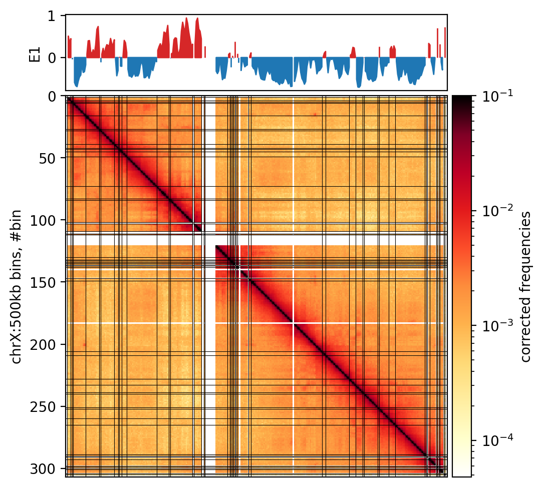

Figure 8.1: chrX interaction matrix with E1 eigenvector values in 500kb resolution. The sign change of the E1 is overlayed as thin black lines, making it more easily interpretable. We should qualitatively determine how well the E1 values capture the plaid pattern in the matrix.

Markdown: Figure 10.1

We observe that the E1 values only somewhat captures the plaid pattern in the matrix Figure 10.1, but it is not related to the size of the compartments, as both small and large compartments can be observed. The B-compartment that starts from around bin 150 (75.000.000 bp) seems to have squares that are not captured by the E1 values. Maybe it could be captures by TAD calling, but that is not the scope of this analysis.

#import matplotlib.pyplot as plt

f, ax1 = plt.subplots(
    figsize=(6, 1),
)

# Fill between the line and 0
ax1.fill_between(range(len(e1X_values)), e1X_values, 0, where=(e1X_values > 0), color='tab:red')
ax1.fill_between(range(len(e1X_values)), e1X_values, 0, where=(e1X_values < 0), color='tab:blue')

#ax1.set_ylabel('E1')
ax1.set_xticks([])
ax1.set_yticks([])

# Remove borders
ax1.spines['top'].set_visible(False)
ax1.spines['right'].set_visible(False)
ax1.spines['left'].set_visible(False)
ax1.spines['bottom'].set_visible(False)

plt.tight_layout()

# Save the plot as a SVG file
#plt.savefig('e1_plot.svg', bbox_inches='tight')

plt.show()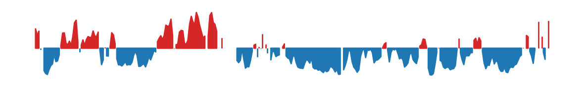

Figure 8.2: 500kb binned E1 eigenvector values for chrX. Freshly calculated from the cooler file.

Markdown the next plot: Figure 10.3 that is

Stairs plot of the E1 compartments

(Less spiky, more smooth)

#import matplotlib.pyplot as plt


f, (ax1, ax2) = plt.subplots(2,1,
    figsize=(6, 2)
)

chrom_start = eigenvector_track_chrX['start'].values
window_size = chrom_start[1] - chrom_start[0]

# Fill between the line and 0
ax1.fill_between(range(len(e1X_values)), e1X_values, 0, where=(e1X_values > 0), color='tab:red')
ax1.fill_between(range(len(e1X_values)), e1X_values, 0, where=(e1X_values < 0), color='tab:blue')

# Create stairs
x = np.zeros(2*chrom_start.size)
y = np.zeros(2*chrom_start.size)
x[0::2] = chrom_start
x[1::2] = chrom_start + window_size
y[0::2] = e1X_values
y[1::2] = e1X_values

# Layout
ax1.set_ylabel('Spiky E1')
ax2.set_ylabel('Stairs E1')
ax1.set_xticks([])
ax1.set_yticks([])
ax2.set_xticks([])
ax2.set_yticks([])
ax2.set_ylim(-1, 1)

# Remove borders
ax1.spines[:].set_visible(False)
ax2.spines[:].set_visible(False)

ax2.fill_between(x, y, 0, where=(y > 0), color='tab:red', ec = 'None')
ax2.fill_between(x, y, 0, where=(y < 0), color='tab:blue', ec = 'None')

plt.tight_layout()
# Save the plot as a high-resolution PNG file
#plt.savefig('../steps/e1_plot.png', dpi=320, bbox_inches='tight')

500kb binned E1 eigenvector values for chrX.

Balanced vs unbalanced matrix

# Plot balanced vs unbalanced

from matplotlib.colors import LogNorm
from mpl_toolkits.axes_grid1 import make_axes_locatable

f, axs = plt.subplots(1, 2,
    figsize=(6, 2),
)
axs = axs.flatten()

#### The unbalanced matrix
ax = axs[0]
norm = LogNorm(vmin=1, vmax=100_000)
im = ax.matshow(
    clr.matrix(balance=False).fetch('chrX'),
    norm=norm,
    cmap='fall',
);
#plt.axis([0,nbins,nbins,0])


divider = make_axes_locatable(ax)
cax = divider.append_axes("right", size="5%", pad=0.05)
plt.colorbar(im, cax=cax);
ax.set_ylabel('#bin (500kb)')
ax.set_title('Unbalanced matrix')
ax.xaxis.set_visible(False)


#### The balanced matrix
ax = axs[1]
norm = LogNorm(vmax=0.1)
im = ax.matshow(
    clr.matrix().fetch('chrX'),
    norm=norm,
    cmap='fall',
);
#plt.axis([0,nbins,nbins,0])


divider = make_axes_locatable(ax)
cax = divider.append_axes("right", size="5%", pad=0.05)
plt.colorbar(im, cax=cax);
ax.set_ylabel('#bin (500kb)')
ax.set_title('Balanced matrix')
ax.xaxis.set_visible(False)

plt.tight_layout()


# for i in np.where(np.diff( (cis_eigs[1][cis_eigs[1]['chrom']=='chrX']['E1']>0).astype(int)))[0]:
#     # Horisontal lines where E1 intersects 0
#     ax.plot([0,nbins],[i,i],'k',lw=0.4)

#     # Vertical lines where E1 intersects 0
#     ax.plot([i,i],[0,nbins],'k',lw=0.4)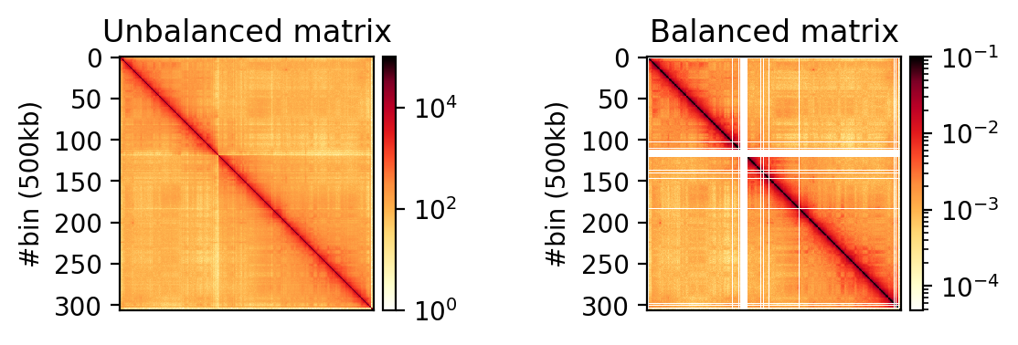

Figure 8.3: Balanced vs unbalanced chrX interaction matrix in 500kb resolution. The balanced matrix is more interpretable, as the colorbar is log-transformed. Balancing also filters out low-count bins, that are otherwise interpreted as low interaction.

Adaptive coarsegrain and interpolation

from matplotlib.colors import LogNorm
from mpl_toolkits.axes_grid1 import make_axes_locatable
from cooltools.lib.numutils import adaptive_coarsegrain, interp_nan

%%capture rs_chrx_raw_balanced_cgi

#| label: fig-rs-chrx-raw-balanced-cgi
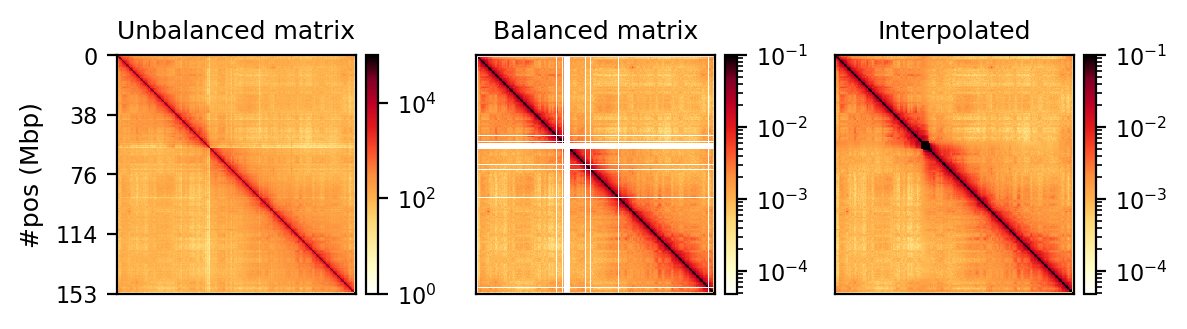
#| fig-cap: "Raw, balanced, and interpolated chrX interaction matrix in 500kb resolution. The interpolation is done to make the matrix more visually appealing, but it is not necessary for the analysis."

clr = cooler.Cooler(f"{mclr}::resolutions/500000")
bins = clr.bins().fetch('chrX')[:].reset_index(drop=True)
yticks = np.linspace(0, bins.shape[0]-1, 5, dtype=int)
yticklabels = [value for value in bins['start'][yticks].values//1_000_000]

f, axs = plt.subplots(1, 3,
    figsize=(6, 2)
)
axs = axs.flatten()

#### The unbalanced matrix
ax = axs[0]
norm = LogNorm(vmin=1, vmax=100_000)
im = ax.matshow(
    clr.matrix(balance=False).fetch('chrX'),
    norm=norm,
    cmap='fall',
);
#plt.axis([0,nbins,nbins,0])


divider = make_axes_locatable(ax)
cax = divider.append_axes("right", size="5%", pad=0.05)
plt.colorbar(im, cax=cax);
ax.set_ylabel('#pos (Mbp)')
ax.set_yticks(yticks)
ax.set_yticklabels(yticklabels)
ax.set_title('Unbalanced matrix')
ax.xaxis.set_visible(False)


#### The balanced matrix
ax = axs[1]
norm = LogNorm(vmax=0.1)
im = ax.matshow(
    clr.matrix().fetch('chrX'),
    norm=norm,
    cmap='fall',
);
#plt.axis([0,nbins,nbins,0])

divider = make_axes_locatable(ax)
cax = divider.append_axes("right", size="5%", pad=0.05)
plt.colorbar(im, cax=cax);
# Remove y-ticks
ax.yaxis.set_visible(False)
ax.set_title('Balanced matrix')
ax.xaxis.set_visible(False)

### Coursegrain and interpolate (beautify)
ax = axs[2]
cg = adaptive_coarsegrain(clr.matrix(balance=True).fetch('chrX'),
                              clr.matrix(balance=False).fetch('chrX'),
                              cutoff=3, max_levels=8)
cgi = interp_nan(cg)

im = ax.matshow(cgi, cmap='fall', norm=norm, rasterized=False)

divider = make_axes_locatable(ax)
cax = divider.append_axes("right", size="5%", pad=0.05)
plt.colorbar(im, cax=cax);
ax.xaxis.set_visible(False)
ax.yaxis.set_visible(False)
ax.set_title(f'Interpolated')

#plt.suptitle('Round Spermatid at 500kb resolution', fontsize=11)
plt.tight_layout()

%%capture rs_chrx_raw_balanced_cgi_subset
#| label: fig-rs-chrx-raw-balanced-cgi-subset
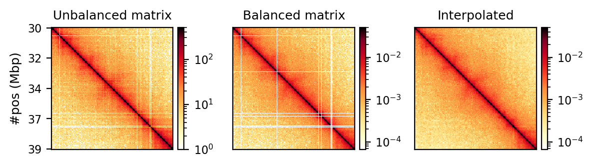
#| fig-cap: "Raw, balanced, and interpolated chrX interaction matrix in 50kb resolution. The interpolation is done to make the matrix more visually appealing, but it is not necessary for the analysis."

# Now with a zoomed in version
clr = cooler.Cooler(f"{mclr}::resolutions/50000")
extent = (30_000_000, 40_000_000)
region = f'chrX:{extent[0]}-{extent[1]}'
bins = clr.bins().fetch(region)[:].reset_index(drop=True)
yticks = np.linspace(0, bins.shape[0]-1, 5, dtype=int)
yticklabels = [value for value in bins['start'][yticks].values//1_000_000]

f, axs = plt.subplots(1, 3,
    figsize=(6, 2)
)
axs = axs.flatten()

#### The unbalanced matrix
ax = axs[0]
norm = LogNorm(vmin=1, vmax=500)
im = ax.matshow(
    clr.matrix(balance=False).fetch(region),
    norm=norm,
    cmap='fall',
    #extent=(extent[0], extent[1], extent[1], extent[0])
);
#plt.axis([0,nbins,nbins,0])
divider = make_axes_locatable(ax)
cax = divider.append_axes("right", size="5%", pad=0.05)
plt.colorbar(im, cax=cax);
ax.set_ylabel('#pos (Mbp)')
ax.set_yticks(yticks)
ax.set_yticklabels(yticklabels)
ax.set_title('Unbalanced matrix')
ax.xaxis.set_visible(False)


#### The balanced matrix
ax = axs[1]
norm = LogNorm(vmax=0.05)
im = ax.matshow(
    clr.matrix().fetch(region),
    norm=norm,
    cmap='fall',
    #extent=(extent[0], extent[1], extent[1], extent[0])
);
#plt.axis([0,nbins,nbins,0])

divider = make_axes_locatable(ax)
cax = divider.append_axes("right", size="5%", pad=0.05)
plt.colorbar(im, cax=cax);
# Remove y-ticks
ax.yaxis.set_visible(False)
ax.set_title('Balanced matrix')
ax.xaxis.set_visible(False)

### Coursegrain and interpolate (beautify)
ax = axs[2]
cg = adaptive_coarsegrain(clr.matrix(balance=True).fetch(region),
                              clr.matrix(balance=False).fetch(region),
                              cutoff=3, max_levels=8)
cgi = interp_nan(cg)

im = ax.matshow(cgi, cmap='fall', norm=norm, 
                #extent=(extent[0], extent[1], extent[1], extent[0])
                )

divider = make_axes_locatable(ax)
cax = divider.append_axes("right", size="5%", pad=0.05)
plt.colorbar(im, cax=cax);
ax.xaxis.set_visible(False)
ax.yaxis.set_visible(False)
ax.set_title(f'Interpolated')

#plt.suptitle('Round Spermatid at 50kb resolution', fontsize=11)
plt.tight_layout()

display(rs_chrx_raw_balanced_cgi.outputs[0],
        rs_chrx_raw_balanced_cgi_subset.outputs[0]
)

(a) Full RS matrix at 500kb resolution

(b) Subset RS matrix at 50kb resolution

Figure 8.4: Raw, balanced, and interpolated chrX interaction matrix in a) 500kb resolution (full chrX) or b) 50kb resolution (chrX:30Mb-39Mb). The interpolation is done to make the matrix more visually appealing, but it is not necessary for the analysis.

500kb resolution

All 5 full merges

Load coolers

import glob
import os.path as op
import cooler

mcools = glob.glob("../steps/bwa/recPE/cool/*/*.mcool")
res = "::resolutions/500000"

clrs = {op.basename(op.dirname(mcool)): cooler.Cooler(mcool+res) for mcool in mcools}

chron_order = ['fibroblast', 'spermatogonia', 'pachytene_spermatocyte', 'round_spermatid', 'sperm']
abbr_list = ['Fb', 'SPA', 'PAC', 'RS', 'SP']
abbr = {key: abbr_list[i] for i,key in enumerate(chron_order)}

clrs = {key: clrs[key] for key in chron_order}
clrs

{'fibroblast': <Cooler "fibroblast.mcool::/resolutions/500000">,
 'spermatogonia': <Cooler "spermatogonia.mcool::/resolutions/500000">,
 'pachytene_spermatocyte': <Cooler "pachytene_spermatocyte.mcool::/resolutions/500000">,
 'round_spermatid': <Cooler "round_spermatid.mcool::/resolutions/500000">,
 'sperm': <Cooler "sperm.mcool::/resolutions/500000">}

Calculate gc covariance (from the reference genome)

Do this with any of the clrs - it just needs the bins positions.

# Try with only the gc_cov for chrX

import bioframe
import pandas as pd
import os.path as op

bins = clrs['fibroblast'].bins().fetch('chrX')[:]
out_name = '../steps/rheMac10_gc_cov_X_500kb.tsv'

rheMac10 = bioframe.load_fasta('../data/links/ucsc_ref/rheMac10.fa')
if not op.exists(out_name):
    print('Calculate the fraction of GC basepairs for each bin')
    gc_cov = bioframe.frac_gc(bins[['chrom', 'start', 'end']], rheMac10)
    gc_cov.to_csv(out_name, index=False,sep='\t')
    print(gc_cov.info())
else: 
    print("Already exists, read from file")
    gc_cov = pd.read_csv(out_name, sep='\t')
    print(gc_cov.info())

Already exists, read from file
<class 'pandas.core.frame.DataFrame'>
RangeIndex: 307 entries, 0 to 306
Data columns (total 4 columns):
 #   Column  Non-Null Count  Dtype  
---  ------  --------------  -----  
 0   chrom   307 non-null    object 
 1   start   307 non-null    int64  
 2   end     307 non-null    int64  
 3   GC      307 non-null    float64
dtypes: float64(1), int64(2), object(1)
memory usage: 9.7+ KB
None

Calculate the E1 compartments

Loop: view_df, cis_eigs, e1_values

Plot GC covariance

import matplotlib.pyplot as plt

f, ax = plt.subplots(
    figsize=(10, 2),
)

ax.plot(gc_cov['start'],gc_cov['GC'])

plt.tight_layout()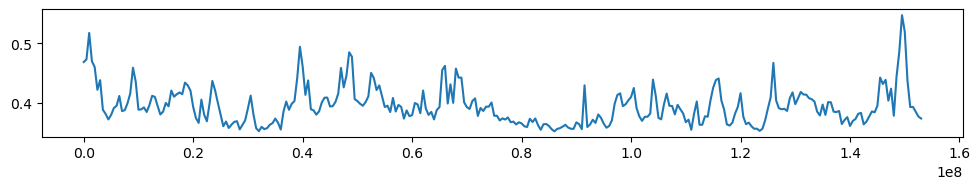

Chromosome restricted E1 compartments

# Use gc_cov to calculate eigenvectors with cooltools.eigs_cis

import cooltools
import pandas as pd

eigs_full = {}
e1_values_full = {}

chrX_size = clrs['fibroblast'].chromsizes['chrX']

# Divide into chromosome arms
clr = clrs['fibroblast']
view_df_full = pd.DataFrame(
    {
    'chrom': 'chrX',
    'start': 0,
    'end': chrX_size,
    'name': 'chrX'
    }, index=[0]
                      )

for name, clr in clrs.items():
    print(f"Calculating eigenvectors for {name}, size {clr.binsize}")
    cis_eigs_full = cooltools.eigs_cis(
                        clr,
                        gc_cov,
                        view_df=view_df_full,
                        n_eigs=3,
                        )
    eigs_full[name] = cis_eigs_full[1]
    e1_track_full = cis_eigs_full[1][['chrom','start','end','E1']]
    e1_values_full[name] = e1_track_full['E1'].values

#eigs

Calculating eigenvectors for fibroblast, size 500000

/home/sojern/miniconda3/envs/hic/lib/python3.12/site-packages/cooltools/lib/common.py:489: UserWarning: less than 50% of valid bins have been assigned a value
  warnings.warn("less than 50% of valid bins have been assigned a value")

Calculating eigenvectors for spermatogonia, size 500000

/home/sojern/miniconda3/envs/hic/lib/python3.12/site-packages/cooltools/lib/common.py:489: UserWarning: less than 50% of valid bins have been assigned a value
  warnings.warn("less than 50% of valid bins have been assigned a value")

Calculating eigenvectors for pachytene_spermatocyte, size 500000

/home/sojern/miniconda3/envs/hic/lib/python3.12/site-packages/cooltools/lib/common.py:489: UserWarning: less than 50% of valid bins have been assigned a value
  warnings.warn("less than 50% of valid bins have been assigned a value")

Calculating eigenvectors for round_spermatid, size 500000

/home/sojern/miniconda3/envs/hic/lib/python3.12/site-packages/cooltools/lib/common.py:489: UserWarning: less than 50% of valid bins have been assigned a value
  warnings.warn("less than 50% of valid bins have been assigned a value")

Calculating eigenvectors for sperm, size 500000

/home/sojern/miniconda3/envs/hic/lib/python3.12/site-packages/cooltools/lib/common.py:489: UserWarning: less than 50% of valid bins have been assigned a value
  warnings.warn("less than 50% of valid bins have been assigned a value")

Chromosome arms restricted

# Use gc_cov to calculate eigenvectors with cooltools.eigs_cis

import cooltools
import pandas as pd

eigs = {}
e1_values = {}

chrX_size = clrs['fibroblast'].chromsizes['chrX']

# Divide into chromosome arms
view_df = pd.DataFrame(
    {
    'chrom': 'chrX',
    'start': [0, 59_000_001],
    'end': [59_000_000, chrX_size],
    'name': ['X_short', 'X_long']
    }, index=[0,1]
                      )

for name, clr in clrs.items():
    print(f"Calculating eigenvectors for {name}")
    cis_eigs = cooltools.eigs_cis(
                        clr,
                        gc_cov,
                        view_df=view_df,
                        n_eigs=3,
                        )
    eigs[name] = cis_eigs[1]
    e1_track = cis_eigs[1][['chrom','start','end','E1']]
    e1_values[name] = e1_track['E1'].values

#eigs

Calculating eigenvectors for fibroblast

/home/sojern/miniconda3/envs/hic/lib/python3.12/site-packages/cooltools/lib/common.py:489: UserWarning: less than 50% of valid bins have been assigned a value
  warnings.warn("less than 50% of valid bins have been assigned a value")

Calculating eigenvectors for spermatogonia

/home/sojern/miniconda3/envs/hic/lib/python3.12/site-packages/cooltools/lib/common.py:489: UserWarning: less than 50% of valid bins have been assigned a value
  warnings.warn("less than 50% of valid bins have been assigned a value")

Calculating eigenvectors for pachytene_spermatocyte
Calculating eigenvectors for round_spermatid

/home/sojern/miniconda3/envs/hic/lib/python3.12/site-packages/cooltools/lib/common.py:489: UserWarning: less than 50% of valid bins have been assigned a value
  warnings.warn("less than 50% of valid bins have been assigned a value")
/home/sojern/miniconda3/envs/hic/lib/python3.12/site-packages/cooltools/lib/common.py:489: UserWarning: less than 50% of valid bins have been assigned a value
  warnings.warn("less than 50% of valid bins have been assigned a value")

Calculating eigenvectors for sperm

/home/sojern/miniconda3/envs/hic/lib/python3.12/site-packages/cooltools/lib/common.py:489: UserWarning: less than 50% of valid bins have been assigned a value
  warnings.warn("less than 50% of valid bins have been assigned a value")

Refined: 10Mb windows restricted

# Use gc_cov to calculate eigenvectors with cooltools.eigs_cis

import cooltools

eigs_10mb = {}
e1_values_10mb = {}

chrX_size = clrs['fibroblast'].chromsizes['chrX']

# Calculate in 10Mb windows
# Define the window size (10Mb)

window_size = 10_000_000

# Generate the start and end positions for each window
start_positions = list(range(0, chrX_size, window_size))
end_positions = [min(start + window_size, chrX_size) for start in start_positions]
# Create the DataFrame
view_df_10mb = pd.DataFrame({
    'chrom': ['chrX'] * len(start_positions),
    'start': start_positions,
    'end': end_positions,
    'name': [f'X_{i}' for i in range(len(start_positions))]
})
#display(view_df)

for name, clr in clrs.items():
    print(f"Calculating eigenvectors for {name}")
    cis_eigs_10mb = cooltools.eigs_cis(
                        clr,
                        gc_cov,
                        view_df=view_df_10mb,
                        n_eigs=3,
                        )
    eigs_10mb[name] = cis_eigs_10mb[1]
    e1_track_10mb = cis_eigs_10mb[1][['chrom','start','end','E1']]
    e1_values_10mb[name] = e1_track_10mb['E1'].values

#eigs

Calculating eigenvectors for fibroblast

/home/sojern/miniconda3/envs/hic/lib/python3.12/site-packages/cooltools/lib/common.py:489: UserWarning: less than 50% of valid bins have been assigned a value
  warnings.warn("less than 50% of valid bins have been assigned a value")

Calculating eigenvectors for spermatogonia

/home/sojern/miniconda3/envs/hic/lib/python3.12/site-packages/cooltools/lib/common.py:489: UserWarning: less than 50% of valid bins have been assigned a value
  warnings.warn("less than 50% of valid bins have been assigned a value")

Calculating eigenvectors for pachytene_spermatocyte

/home/sojern/miniconda3/envs/hic/lib/python3.12/site-packages/cooltools/lib/common.py:489: UserWarning: less than 50% of valid bins have been assigned a value
  warnings.warn("less than 50% of valid bins have been assigned a value")

Calculating eigenvectors for round_spermatid

/home/sojern/miniconda3/envs/hic/lib/python3.12/site-packages/cooltools/lib/common.py:489: UserWarning: less than 50% of valid bins have been assigned a value
  warnings.warn("less than 50% of valid bins have been assigned a value")

Calculating eigenvectors for sperm

/home/sojern/miniconda3/envs/hic/lib/python3.12/site-packages/cooltools/lib/common.py:489: UserWarning: less than 50% of valid bins have been assigned a value
  warnings.warn("less than 50% of valid bins have been assigned a value")

Save the A compartment coordinates, also E1 track

######## Restriction: chromosome arm E1 values ########
import importlib
import hicstuff
import os
importlib.reload(hicstuff)
from hicstuff import extract_a_coordinates


# Binsize in bp
res = 500_000
outdir = '../results/rec_compartments/'
if not os.path.exists(outdir):
    os.makedirs(outdir)
    

######## Restriction: full chromosome E1 values ########
restriction = 'full'
for name, e1 in e1_values_full.items():
    extract_a_coordinates(e1=e1, name=name, restriction=restriction, chrom='chrX', res=500_000, csv=True,output_dir=outdir, force=True)

######## Restriction: chromosome arm E1 values ########
restriction = 'arms'
for name, e1 in e1_values.items():
    extract_a_coordinates(e1=e1, name=name, restriction=restriction, chrom='chrX', res=500_000, csv=True,output_dir=outdir, force=True)

######## Restriction: 10Mb E1 values ########
restriction = '10Mb'
for name, e1 in e1_values_10mb.items():
    extract_a_coordinates(e1=e1, name=name, restriction=restriction, chrom='chrX', res=500_000, csv=True,output_dir=outdir, force=True)

Saving eigenvector track to: ../results/rec_compartments/fibroblast_e1_500kb_full.csv
File ../results/rec_compartments/fibroblast_e1_500kb_full.csv already exists. Overwriting.
Calculating A-compartment intervals for fibroblast
File ../results/rec_compartments/fibroblast_a_comp_coords_500kb_full.csv already exists. Overwriting.
Saving eigenvector track to: ../results/rec_compartments/spermatogonia_e1_500kb_full.csv
File ../results/rec_compartments/spermatogonia_e1_500kb_full.csv already exists. Overwriting.
Calculating A-compartment intervals for spermatogonia
File ../results/rec_compartments/spermatogonia_a_comp_coords_500kb_full.csv already exists. Overwriting.
Saving eigenvector track to: ../results/rec_compartments/pachytene_spermatocyte_e1_500kb_full.csv
File ../results/rec_compartments/pachytene_spermatocyte_e1_500kb_full.csv already exists. Overwriting.
Calculating A-compartment intervals for pachytene_spermatocyte
File ../results/rec_compartments/pachytene_spermatocyte_a_comp_coords_500kb_full.csv already exists. Overwriting.
Saving eigenvector track to: ../results/rec_compartments/round_spermatid_e1_500kb_full.csv
File ../results/rec_compartments/round_spermatid_e1_500kb_full.csv already exists. Overwriting.
Calculating A-compartment intervals for round_spermatid
File ../results/rec_compartments/round_spermatid_a_comp_coords_500kb_full.csv already exists. Overwriting.
Saving eigenvector track to: ../results/rec_compartments/sperm_e1_500kb_full.csv
File ../results/rec_compartments/sperm_e1_500kb_full.csv already exists. Overwriting.
Calculating A-compartment intervals for sperm
File ../results/rec_compartments/sperm_a_comp_coords_500kb_full.csv already exists. Overwriting.
Saving eigenvector track to: ../results/rec_compartments/fibroblast_e1_500kb_arms.csv
File ../results/rec_compartments/fibroblast_e1_500kb_arms.csv already exists. Overwriting.
Calculating A-compartment intervals for fibroblast
File ../results/rec_compartments/fibroblast_a_comp_coords_500kb_arms.csv already exists. Overwriting.
Saving eigenvector track to: ../results/rec_compartments/spermatogonia_e1_500kb_arms.csv
File ../results/rec_compartments/spermatogonia_e1_500kb_arms.csv already exists. Overwriting.
Calculating A-compartment intervals for spermatogonia
File ../results/rec_compartments/spermatogonia_a_comp_coords_500kb_arms.csv already exists. Overwriting.
Saving eigenvector track to: ../results/rec_compartments/pachytene_spermatocyte_e1_500kb_arms.csv
File ../results/rec_compartments/pachytene_spermatocyte_e1_500kb_arms.csv already exists. Overwriting.
Calculating A-compartment intervals for pachytene_spermatocyte
File ../results/rec_compartments/pachytene_spermatocyte_a_comp_coords_500kb_arms.csv already exists. Overwriting.
Saving eigenvector track to: ../results/rec_compartments/round_spermatid_e1_500kb_arms.csv
File ../results/rec_compartments/round_spermatid_e1_500kb_arms.csv already exists. Overwriting.
Calculating A-compartment intervals for round_spermatid
File ../results/rec_compartments/round_spermatid_a_comp_coords_500kb_arms.csv already exists. Overwriting.
Saving eigenvector track to: ../results/rec_compartments/sperm_e1_500kb_arms.csv
File ../results/rec_compartments/sperm_e1_500kb_arms.csv already exists. Overwriting.
Calculating A-compartment intervals for sperm
File ../results/rec_compartments/sperm_a_comp_coords_500kb_arms.csv already exists. Overwriting.
Saving eigenvector track to: ../results/rec_compartments/fibroblast_e1_500kb_10Mb.csv
File ../results/rec_compartments/fibroblast_e1_500kb_10Mb.csv already exists. Overwriting.
Calculating A-compartment intervals for fibroblast
File ../results/rec_compartments/fibroblast_a_comp_coords_500kb_10Mb.csv already exists. Overwriting.
Saving eigenvector track to: ../results/rec_compartments/spermatogonia_e1_500kb_10Mb.csv
File ../results/rec_compartments/spermatogonia_e1_500kb_10Mb.csv already exists. Overwriting.
Calculating A-compartment intervals for spermatogonia
File ../results/rec_compartments/spermatogonia_a_comp_coords_500kb_10Mb.csv already exists. Overwriting.
Saving eigenvector track to: ../results/rec_compartments/pachytene_spermatocyte_e1_500kb_10Mb.csv
File ../results/rec_compartments/pachytene_spermatocyte_e1_500kb_10Mb.csv already exists. Overwriting.
Calculating A-compartment intervals for pachytene_spermatocyte
File ../results/rec_compartments/pachytene_spermatocyte_a_comp_coords_500kb_10Mb.csv already exists. Overwriting.
Saving eigenvector track to: ../results/rec_compartments/round_spermatid_e1_500kb_10Mb.csv
File ../results/rec_compartments/round_spermatid_e1_500kb_10Mb.csv already exists. Overwriting.
Calculating A-compartment intervals for round_spermatid
File ../results/rec_compartments/round_spermatid_a_comp_coords_500kb_10Mb.csv already exists. Overwriting.
Saving eigenvector track to: ../results/rec_compartments/sperm_e1_500kb_10Mb.csv
File ../results/rec_compartments/sperm_e1_500kb_10Mb.csv already exists. Overwriting.
Calculating A-compartment intervals for sperm
File ../results/rec_compartments/sperm_a_comp_coords_500kb_10Mb.csv already exists. Overwriting.

Plot NaN histogram

# Check the number of NaN values in the E1 column and create a DataFrame
nan_counts = {k: {'length': len(v), 'NaNs': np.isnan(v).sum()} for k, v in e1_values.items()}
#display(pd.DataFrame.from_dict(nan_counts, orient='index'))

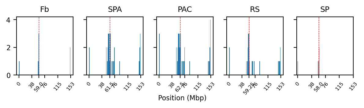
# Locate the NaN values (histogram)
#import matplotlib.pyplot as plt

f, ax = plt.subplots(1, 5, figsize=(6,1.8), sharey=True) # dont share x as they have a different median tick!!!
for i, (name, track) in enumerate(eigs.items()):
    e1 = track['E1'].values
    # Locate NaN values
    e1_nan = np.where(np.isnan(e1))
    # Plot histogram
    ax[i].hist(e1_nan, bins=100)
    
    # Plot median line
    median_pos = np.median(e1_nan) # (1Mb/500Kb) account for binning (res=500kb, target 1Mb y-axis)
#    mean_pos = round(np.mean(e1_nan), 2)
    ax[i].axvline(median_pos, color='r', lw=0.5, ls='--')
#    ax[i].axvline(mean_pos, color='g', lw=0.5, ls='--')

    # Layout
    ax[i].set_title(abbr[name])
    xticks = np.linspace(0, len(e1), num=5)
    xticks = np.append(xticks, median_pos)  # Add median position to xticks
#    xticks = np.append(xticks, mean_pos)  # Add mean position to xticks
    ax[i].set_xticks(xticks)
    xticklabels = np.linspace(0, len(e1) * 0.5, num=5, dtype = 'int').tolist()
    xticklabels.append(median_pos*0.5)  # Add median label
#    xticklabels.append(mean_pos*0.5)  # Add mean label
    ax[i].set_xticklabels(xticklabels, rotation=50, fontsize=6)
    #ax[i].set_xlabel('Position (Mbp)')

plt.tight_layout(rect=[0, 0, 1, 0.95])
f.supxlabel('Position (Mbp)')
plt.show()
                    

Figure 8.5: Histogram of NaN values in the E1 eigenvector for each cell type. Median position is marked with a red dashed line.

Plot the E1 compartments

import matplotlib.pyplot as plt
import numpy as np
from matplotlib.colors import LogNorm
from mpl_toolkits.axes_grid1 import make_axes_locatable
from matplotlib.patches import Rectangle

res = 500_000
names_abbr = {'fibroblast': 'Fibroblast', 'spermatogonia': 'Spermatogonia', 'pachytene_spermatocyte': 'Pachytene Spermatogonia', 'round_spermatid': 'Round Spermatid', 'sperm': 'Sperm'}

chrom_start = e1_track_full['start'].values
chrom_end = e1_track_full['end'].values-1

f, axs = plt.subplots(5, 3, figsize=(18, 8), sharex=True, sharey=True)

# Populate the first column
axs[0,0].set_title('E1: Full-chromosome restricted')
for i, (name, e1) in enumerate(e1_values_full.items()):
    ax = axs[i,0]
    ax.set_ylabel(names_abbr[name])

    #ax.set_title(name)
    
    # Create stairs
    x = np.zeros(2*chrom_start.size)
    y = np.zeros(2*chrom_start.size)
    x[0::2] = chrom_start
    x[1::2] = chrom_end
    y[0::2] = e1
    y[1::2] = e1

    ax.fill_between(x, y, 0, where=(y > 0), color='tab:red', linewidth=0)
    ax.fill_between(x, y, 0, where=(y < 0), color='tab:blue', linewidth=0)

    # Test to see how well my coordinates match the e1 values
    coords = pd.read_csv(f'../results/compartments/{name}_a_comp_coords_500kb_full.csv')
    # Iterate over each interval in the DataFrame
    for start, end in zip(coords['start'], coords['end']):
        rect = Rectangle((start, 0.2), width=end-start, height=0.05, color='k', linewidth=0.05)
        ax.add_patch(rect)

# Populate the second column
axs[0,1].set_title('E1: Chromosome-arms restricted')
for i, (name, e1) in enumerate(e1_values.items()):
    ax = axs[i,1]
    #ax.set_title(name)
    
    # Create stairs
    x = np.zeros(2*chrom_start.size)
    y = np.zeros(2*chrom_start.size)
    x[0::2] = chrom_start
    x[1::2] = chrom_end
    y[0::2] = e1
    y[1::2] = e1

    ax.fill_between(x, y, 0, where=(y > 0), color='tab:red', linewidth=0)
    ax.fill_between(x, y, 0, where=(y < 0), color='tab:blue', linewidth=0)

    # Test to see how well my coordinates match the e1 values
    coords = pd.read_csv(f'../results/compartments/{name}_a_comp_coords_500kb_arms.csv')
    # Iterate over each interval in the DataFrame
    for start, end in zip(coords['start'], coords['end']):
        rect = Rectangle((start, 0.2), width=end-start, height=0.05, color='k', linewidth=0.05)
        ax.add_patch(rect)

# Populate the third column
axs[0,2].set_title('E1: 10Mb restricted (refined)')
for i, (name, e1) in enumerate(e1_values_10mb.items()):
    ax = axs[i,2]
    #ax.set_title(name)
    
    # Create stairs
    x = np.zeros(2*chrom_start.size)
    y = np.zeros(2*chrom_start.size)
    x[0::2] = chrom_start
    x[1::2] = chrom_end
    y[0::2] = e1
    y[1::2] = e1

    ax.fill_between(x, y, 0, where=(y > 0), color='tab:red', ec='None')
    ax.fill_between(x, y, 0, where=(y < 0), color='tab:blue', ec='None')

    # Test to see how well my coordinates match the e1 values
    coords = pd.read_csv(f'../results/compartments/{name}_a_comp_coords_500kb_10Mb.csv')
    # Iterate over each interval in the DataFrame
    for start, end in zip(coords['start'], coords['end']):
        rect = Rectangle((start, 0.2), width=end-start, height=0.05, color='k', linewidth=0.05)
        ax.add_patch(rect)

# Set y-limits for all subplots
for ax in axs.flat:
    ax.set_ylim(-0.8, 0.8)
    ax.spines[:].set_visible(False)
    ax.set_yticks([])
    ax.set_xticks([])

plt.tight_layout()
plt.savefig('../steps/rec_e1_plot_full.svg', bbox_inches='tight')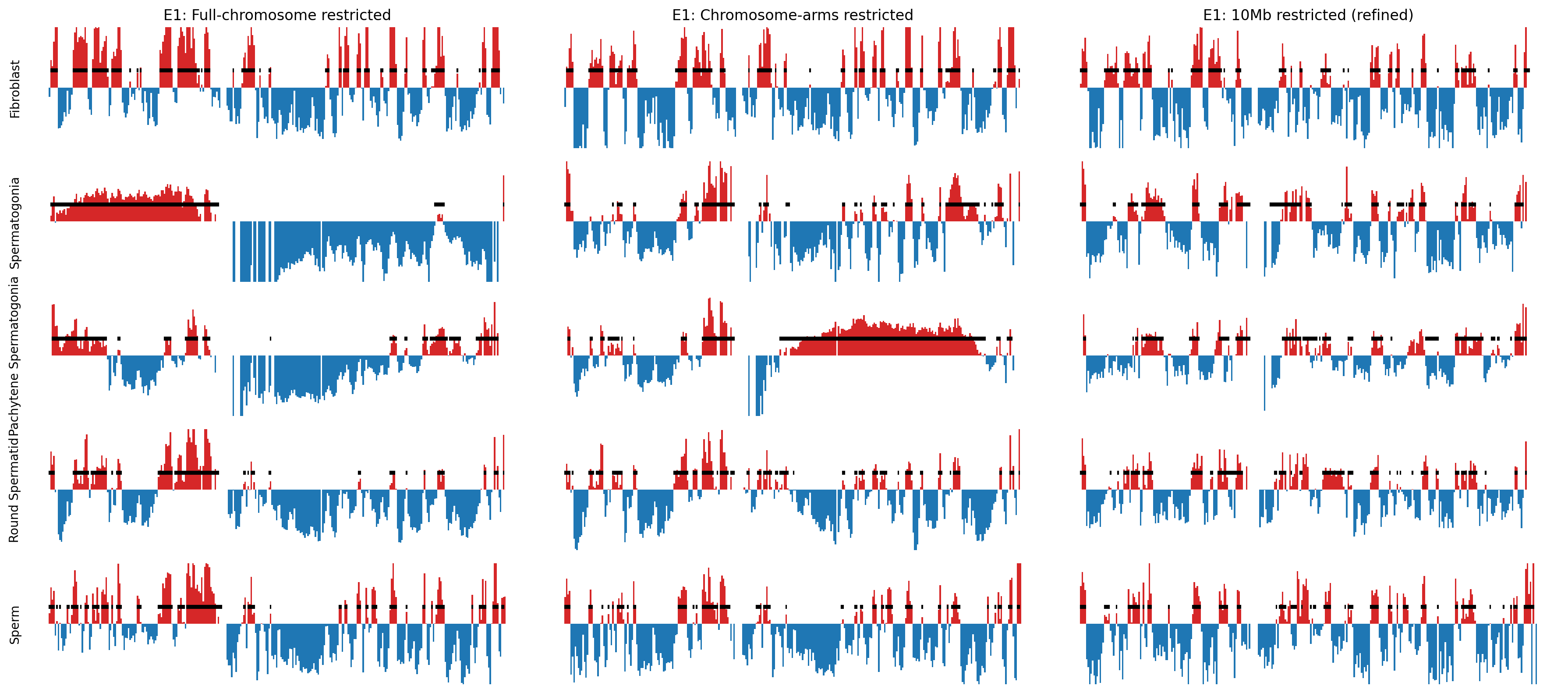

E1 eigenvector values for all merged samples at 500kb resolution. Left: Chromosome-arm restricted E1. Right: 10Mb window restricted E1.

Plot matrices with compartments (round spermatid)

import cooltools.lib.plotting
from matplotlib.colors import LogNorm
from mpl_toolkits.axes_grid1 import make_axes_locatable
from cooltools.lib.numutils import adaptive_coarsegrain, interp_nan



clr = clrs['round_spermatid']
chrom_start, chrom_end = e1_track_full['start'].values, e1_track_full['end'].values-1
e1 = e1_values_10mb['round_spermatid']
nbins = len(clr.bins().fetch('chrX'))

f, ax = plt.subplots(
    figsize=(3,3),
)

norm = LogNorm(vmax=0.1)

e1_list = [e1_values_10mb['round_spermatid'], e1_values['round_spermatid'], e1_values_full['round_spermatid']]
e1_names = ['10Mb', 'Arms', 'Full']
colors = ['tab:red', 'tab:blue', 'tab:green']

# ### Coursegrain and interpolate (beautify)
# cg = adaptive_coarsegrain(clr.matrix(balance=True).fetch('chrX'),
#                           clr.matrix(balance=False).fetch('chrX'),
#                           cutoff=3, max_levels=8, )
# cgi = interp_nan(cg, method='nearest')

im = ax.matshow(
    clr.matrix().fetch('chrX'),
    norm=norm,
    cmap='fall',
);
plt.axis([0,nbins,nbins,0])


divider = make_axes_locatable(ax)
cax = divider.append_axes("right", size="4%", pad=0.05)
plt.colorbar(im, cax=cax, label='Corrected frequencies')
ax.set_ylabel('Position (Mbp)')
ax.xaxis.set_visible(False)
yticks = np.linspace(0, nbins, 5, dtype=int)
yticklabels = yticks*500_000//1_000_000
ax.set_yticks(yticks)
ax.set_yticklabels(yticklabels)



for i, e1 in enumerate(e1_list):
    ax1 = divider.append_axes("top", size="10%", pad=0.05, sharex = ax)

    # Create stairs
    x = np.zeros(2*chrom_start.size)
    y = np.zeros(2*chrom_start.size)
    #smooth_y = np.zeros(2*chrom_start.size)
    x[0::2] = chrom_start/500_000
    x[1::2] = chrom_end/500_000
    y[0::2] = e1
    y[1::2] = e1
    # smooth_e1 = (lambda x: x.rolling(5, 1, center=True).sum())(pd.DataFrame(e1, columns=['value']))['value'].values
    # smooth_y[0::2] = smooth_e1
    # smooth_y[1::2] = smooth_e1


    ax1.fill_between(x, y, 0, where=(y > 0), color='tab:red', ec='None')
    ax1.fill_between(x, y, 0, where=(y < 0), color='tab:blue', ec='None')

    ax1.set_ylabel(e1_names[i], rotation=0, labelpad=5, ha='right', va='center')
    ax1.set_ylim(-0.8, 0.8)
    ax1.set_xticks([])
    ax1.set_yticks([])

    # if e1_names[i] == '10Mb':
    #     # Plot the sign changes on the matrix 
    #     col = 'k' #colors[i]
    #     for i in np.where(np.diff( (pd.Series(e1)>0).astype(int)))[0]:
    #         # Horisontal lines where E1 intersects 0
    #         ax.plot([0,nbins],[i,i],col,lw=0.5)

    #         # Vertical lines where E1 intersects 0
    #         ax.plot([i,i],[0,nbins],col,lw=0.2)

ax1.set_title('Round Spermatid: 500kb bins')
plt.tight_layout()
plt.show()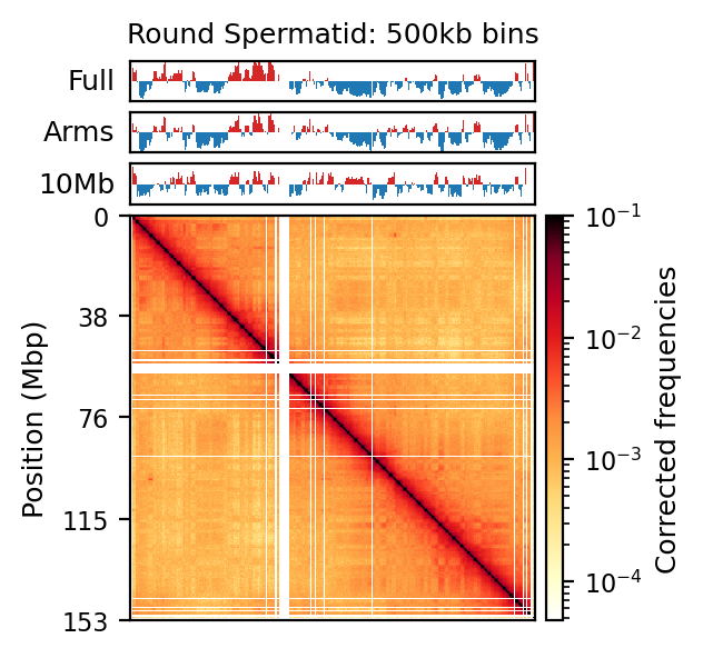

Figure 8.6: E1 eigenvector values for merged round spermatid samples at 500kb resolution, as well as the interaction matrix. E1 was restricted to either Full-chromosome (top), Chromosome-arms (middle), or 10Mb windows (bottom).

Sliding window summed E1 compartments

To mimic the smoothing applied in the Wang et al. 2019 paper, where they slide a 400kb window in 100kb steps on the obs/exp matrix, we will similarly slide a 400kb window in 100kb steps directly on the E1 compartments.

import matplotlib.pyplot as plt
import numpy as np
from matplotlib.colors import LogNorm
from mpl_toolkits.axes_grid1 import make_axes_locatable
import pandas as pd
from scipy.signal.windows import triang

resolution = 500_000
window_size = 2_500_000
step_size = window_size // resolution

chrom_start = e1_track['start'].values
chrom_end = e1_track['end'].values-1

f, axs = plt.subplots(5, 2, figsize=(30, 10), sharex=True)

axs[0, 0].set_title('Chromosome-arm E1 (arm restricted)')
axs[0, 1].set_title('Smoothed by summation')

for i, (name, e1) in enumerate(e1_values.items()):
    # print(i, name, e1.size)
    smooth_e1 = (lambda x: x.rolling(5, 1, center=True).sum())(pd.DataFrame(e1, columns=['value']))

    ax0 = axs[i, 0]
    ax1 = axs[i, 1]
    
    # Create stairs
    x = np.zeros(2*chrom_start.size)
    y = np.zeros(2*chrom_start.size)
    smooth_y = np.zeros(2*chrom_start.size)
    x[0::2] = chrom_start
    x[1::2] = chrom_end
    y[0::2] = e1
    y[1::2] = e1
    smooth_y[0::2] = smooth_e1['value'].values
    smooth_y[1::2] = smooth_e1['value'].values


    ax0.fill_between(x, y, 0, where=(y > 0), color='tab:red')
    ax0.fill_between(x, y, 0, where=(y < 0), color='tab:blue')
    
    # Overlay the smoothed line (divided by 5 to make it a mean)
    ax0.plot(x, smooth_y/5, color='C1')

    ax1.fill_between(x, smooth_y, 0, where=(smooth_y > 0), color='tab:red')
    ax1.fill_between(x, smooth_y, 0, where=(smooth_y < 0), color='tab:blue')

    ax0.set_ylabel(name)
    ylim = 1.5
    #ax0.set_ylim(-ylim, ylim)
    #ax1.set_ylim(-ylim*4, ylim*4)

for ax in axs.flat:
    ax.spines[:].set_visible(False)
    ax.set_xticks([])
    #ax.set_yticks([])

# plt.tight_layout()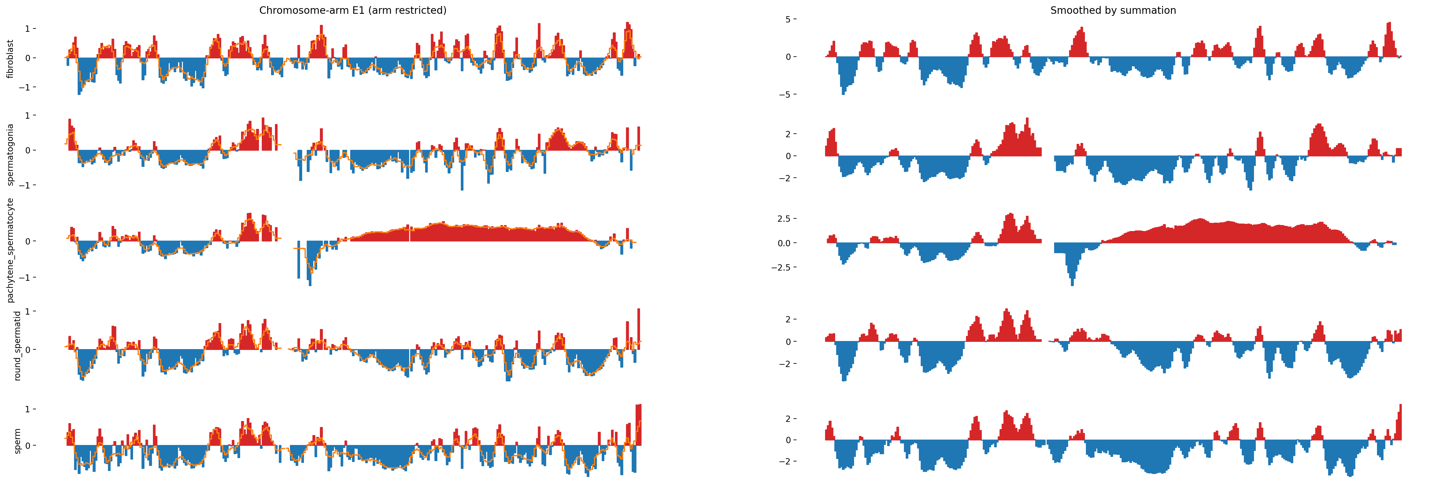

E1 eigenvector values for all merged samples at 500kb resolution with rolling summation, with window size 2.5Mb, step size 500Kb: Each value is now the sum of the surrounding n=5 bins.

100kb resolution

All 5 full merges

Load coolers

import glob
import os.path as op
import cooler

mcools = glob.glob("../steps/bwa/recPE/cool/*/*.mcool")
res = "::resolutions/100000"

clrs = {op.basename(op.dirname(mcool)): cooler.Cooler(mcool+res) for mcool in mcools}

chron_order = ['fibroblast', 'spermatogonia', 'pachytene_spermatocyte', 'round_spermatid', 'sperm']

clrs = {key: clrs[key] for key in chron_order}
clrs

names_abbr = {'fibroblast': 'Fib', 'spermatogonia': 'SPA', 'pachytene_spermatocyte': 'PAC', 'round_spermatid': 'RS', 'sperm': 'Sp'}

# Calculate chromstart and chromend for each bin on chrX
chrX_size = clrs['fibroblast'].chromsizes['chrX']
chrom_start = clrs['fibroblast'].bins().fetch('chrX')['start'].values
chrom_end = clrs['fibroblast'].bins().fetch('chrX')['end'].values-1
nbins = len(clrs['fibroblast'].bins().fetch('chrX'))
binsize = clrs['fibroblast'].binsize

Calculate gc covariance (from the reference genome)

Do this with any of the clrs - it just needs the bins positions.

# Try with only the gc_cov for chrX

import bioframe
import pandas as pd
import os.path as op

bins = clrs['fibroblast'].bins().fetch('chrX')[:]
out_name = '../steps/rheMac10_gc_cov_X_100kb.tsv'

rheMac10 = bioframe.load_fasta('../data/links/ucsc_ref/rheMac10.fa')
if not op.exists(out_name):
    print('Calculate the fraction of GC basepairs for each bin')
    gc_cov = bioframe.frac_gc(bins[['chrom', 'start', 'end']], rheMac10)
    gc_cov.to_csv(out_name, index=False,sep='\t')
    print(gc_cov.info())
else: 
    print("Already exists, read from file")
    gc_cov = pd.read_csv(out_name, sep='\t')
    print(gc_cov.info())

Already exists, read from file
<class 'pandas.core.frame.DataFrame'>
RangeIndex: 1534 entries, 0 to 1533
Data columns (total 4 columns):
 #   Column  Non-Null Count  Dtype  
---  ------  --------------  -----  
 0   chrom   1534 non-null   object 
 1   start   1534 non-null   int64  
 2   end     1534 non-null   int64  
 3   GC      1533 non-null   float64
dtypes: float64(1), int64(2), object(1)
memory usage: 48.1+ KB
None

Calculate the E1 compartments

Loop: view_df, cis_eigs, e1_values

Plot GC covariance

import matplotlib.pyplot as plt


f, ax = plt.subplots(figsize=(10, 2))

ax.plot(gc_cov['start'],gc_cov['GC'])
plt.tight_layout()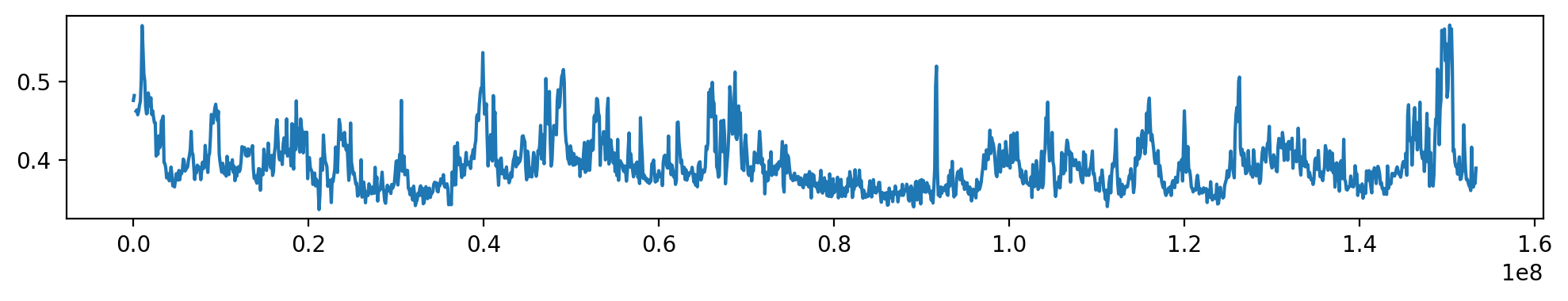

Create viewframes: full, arms, 10Mb windows

import pandas as pd

# Fetch the chromsize of X from one of the coolers
chrX_size = clrs['fibroblast'].chromsizes['chrX']

views = {}

# Make the full view frame
views['full'] = pd.DataFrame({
    'chrom': 'chrX',
    'start': 0,
    'end': chrX_size,
    'name': 'chrX'}, index=[0])

# Divide into chromosome arms
views['arms'] = pd.DataFrame({
    'chrom': 'chrX',
    'start': [0, 59_000_001],
    'end': [59_000_000, chrX_size],
    'name': ['X_short', 'X_long']}, index=[0,1])

# Calculate in 10Mb windows
window_size = 10_000_000
start_positions = list(range(0, chrX_size, window_size))
end_positions = [min(start + window_size, chrX_size) for start in start_positions]

# Create the DataFrame
views['10Mb'] = pd.DataFrame({
    'chrom': ['chrX'] * len(start_positions),
    'start': start_positions,
    'end': end_positions,
    'name': [f'X_{i}' for i in range(len(start_positions))]
})

Calulate the E1 compartments

import cooltools

eigs = {}
e1_values = {}

for name, clr in clrs.items():
    if name not in eigs or name not in e1_values:
        eigs[name] = {} 
        e1_values[name] = {}
    for view, view_df in views.items():
        print(f"Calculating eigenvectors for {name} at {view}")
        cis_eigs = cooltools.eigs_cis(
                            clr,
                            gc_cov,
                            view_df=view_df,
                            n_eigs=1)
        eigs[name][view] = cis_eigs[1]
        e1_values[name][view] = cis_eigs[1]['E1'].values
        

Calculating eigenvectors for fibroblast at full

/home/sojern/miniconda3/envs/hic/lib/python3.12/site-packages/cooltools/lib/common.py:489: UserWarning: less than 50% of valid bins have been assigned a value
  warnings.warn("less than 50% of valid bins have been assigned a value")

Calculating eigenvectors for fibroblast at arms

/home/sojern/miniconda3/envs/hic/lib/python3.12/site-packages/cooltools/lib/common.py:489: UserWarning: less than 50% of valid bins have been assigned a value
  warnings.warn("less than 50% of valid bins have been assigned a value")

Calculating eigenvectors for fibroblast at 10Mb

/home/sojern/miniconda3/envs/hic/lib/python3.12/site-packages/cooltools/lib/common.py:489: UserWarning: less than 50% of valid bins have been assigned a value
  warnings.warn("less than 50% of valid bins have been assigned a value")

Calculating eigenvectors for spermatogonia at full

/home/sojern/miniconda3/envs/hic/lib/python3.12/site-packages/cooltools/lib/common.py:489: UserWarning: less than 50% of valid bins have been assigned a value
  warnings.warn("less than 50% of valid bins have been assigned a value")

Calculating eigenvectors for spermatogonia at arms

/home/sojern/miniconda3/envs/hic/lib/python3.12/site-packages/cooltools/lib/common.py:489: UserWarning: less than 50% of valid bins have been assigned a value
  warnings.warn("less than 50% of valid bins have been assigned a value")

Calculating eigenvectors for spermatogonia at 10Mb

/home/sojern/miniconda3/envs/hic/lib/python3.12/site-packages/cooltools/lib/common.py:489: UserWarning: less than 50% of valid bins have been assigned a value
  warnings.warn("less than 50% of valid bins have been assigned a value")

Calculating eigenvectors for pachytene_spermatocyte at full

/home/sojern/miniconda3/envs/hic/lib/python3.12/site-packages/cooltools/lib/common.py:489: UserWarning: less than 50% of valid bins have been assigned a value
  warnings.warn("less than 50% of valid bins have been assigned a value")

Calculating eigenvectors for pachytene_spermatocyte at arms

/home/sojern/miniconda3/envs/hic/lib/python3.12/site-packages/cooltools/lib/common.py:489: UserWarning: less than 50% of valid bins have been assigned a value
  warnings.warn("less than 50% of valid bins have been assigned a value")

Calculating eigenvectors for pachytene_spermatocyte at 10Mb

/home/sojern/miniconda3/envs/hic/lib/python3.12/site-packages/cooltools/lib/common.py:489: UserWarning: less than 50% of valid bins have been assigned a value
  warnings.warn("less than 50% of valid bins have been assigned a value")

Calculating eigenvectors for round_spermatid at full

/home/sojern/miniconda3/envs/hic/lib/python3.12/site-packages/cooltools/lib/common.py:489: UserWarning: less than 50% of valid bins have been assigned a value
  warnings.warn("less than 50% of valid bins have been assigned a value")

Calculating eigenvectors for round_spermatid at arms

/home/sojern/miniconda3/envs/hic/lib/python3.12/site-packages/cooltools/lib/common.py:489: UserWarning: less than 50% of valid bins have been assigned a value
  warnings.warn("less than 50% of valid bins have been assigned a value")

Calculating eigenvectors for round_spermatid at 10Mb

/home/sojern/miniconda3/envs/hic/lib/python3.12/site-packages/cooltools/lib/common.py:489: UserWarning: less than 50% of valid bins have been assigned a value
  warnings.warn("less than 50% of valid bins have been assigned a value")

Calculating eigenvectors for sperm at full

/home/sojern/miniconda3/envs/hic/lib/python3.12/site-packages/cooltools/lib/common.py:489: UserWarning: less than 50% of valid bins have been assigned a value
  warnings.warn("less than 50% of valid bins have been assigned a value")

Calculating eigenvectors for sperm at arms

/home/sojern/miniconda3/envs/hic/lib/python3.12/site-packages/cooltools/lib/common.py:489: UserWarning: less than 50% of valid bins have been assigned a value
  warnings.warn("less than 50% of valid bins have been assigned a value")

Calculating eigenvectors for sperm at 10Mb

/home/sojern/miniconda3/envs/hic/lib/python3.12/site-packages/cooltools/lib/common.py:489: UserWarning: less than 50% of valid bins have been assigned a value
  warnings.warn("less than 50% of valid bins have been assigned a value")

Extract the A compartment coordinates as well as E1 track

import importlib
import hicstuff
importlib.reload(hicstuff)
from hicstuff import extract_a_coordinates


res = 100_000
outdir = '../results/rec_compartments/'

for name, view_df in e1_values.items():
    print(f"Calculating A-compartment intervals for {name}")
    for view, e1 in view_df.items():
        print(view)
        extract_a_coordinates(
            e1=e1,
            name=name,
            restriction=view,
            chrom='chrX',
            res=res,
            csv=True,
            output_dir=outdir,
            force=True
        )
        extract_a_coordinates(
            e1=e1,
            name=name,
            restriction=view,
            chrom='chrX',
            res=res,
            csv=True,
            output_dir=outdir,
            smooth=True,
            force=True
        )
    

Calculating A-compartment intervals for fibroblast
full
Saving eigenvector track to: ../results/rec_compartments/fibroblast_e1_100kb_full.csv
File ../results/rec_compartments/fibroblast_e1_100kb_full.csv already exists. Overwriting.
Calculating A-compartment intervals for fibroblast
File ../results/rec_compartments/fibroblast_a_comp_coords_100kb_full.csv already exists. Overwriting.
Saving eigenvector track to: ../results/rec_compartments/fibroblast_e1_100kb_full_smoothed.csv
Calculating A-compartment intervals for fibroblast
File ../results/rec_compartments/fibroblast_a_comp_coords_100kb_full_smoothed.csv already exists. Overwriting.
arms
Saving eigenvector track to: ../results/rec_compartments/fibroblast_e1_100kb_arms.csv
File ../results/rec_compartments/fibroblast_e1_100kb_arms.csv already exists. Overwriting.
Calculating A-compartment intervals for fibroblast
File ../results/rec_compartments/fibroblast_a_comp_coords_100kb_arms.csv already exists. Overwriting.
Saving eigenvector track to: ../results/rec_compartments/fibroblast_e1_100kb_arms_smoothed.csv
Calculating A-compartment intervals for fibroblast
File ../results/rec_compartments/fibroblast_a_comp_coords_100kb_arms_smoothed.csv already exists. Overwriting.
10Mb
Saving eigenvector track to: ../results/rec_compartments/fibroblast_e1_100kb_10Mb.csv
File ../results/rec_compartments/fibroblast_e1_100kb_10Mb.csv already exists. Overwriting.
Calculating A-compartment intervals for fibroblast
File ../results/rec_compartments/fibroblast_a_comp_coords_100kb_10Mb.csv already exists. Overwriting.
Saving eigenvector track to: ../results/rec_compartments/fibroblast_e1_100kb_10Mb_smoothed.csv
Calculating A-compartment intervals for fibroblast
File ../results/rec_compartments/fibroblast_a_comp_coords_100kb_10Mb_smoothed.csv already exists. Overwriting.
Calculating A-compartment intervals for spermatogonia
full
Saving eigenvector track to: ../results/rec_compartments/spermatogonia_e1_100kb_full.csv
File ../results/rec_compartments/spermatogonia_e1_100kb_full.csv already exists. Overwriting.
Calculating A-compartment intervals for spermatogonia
File ../results/rec_compartments/spermatogonia_a_comp_coords_100kb_full.csv already exists. Overwriting.
Saving eigenvector track to: ../results/rec_compartments/spermatogonia_e1_100kb_full_smoothed.csv
Calculating A-compartment intervals for spermatogonia
File ../results/rec_compartments/spermatogonia_a_comp_coords_100kb_full_smoothed.csv already exists. Overwriting.
arms
Saving eigenvector track to: ../results/rec_compartments/spermatogonia_e1_100kb_arms.csv
File ../results/rec_compartments/spermatogonia_e1_100kb_arms.csv already exists. Overwriting.
Calculating A-compartment intervals for spermatogonia
File ../results/rec_compartments/spermatogonia_a_comp_coords_100kb_arms.csv already exists. Overwriting.
Saving eigenvector track to: ../results/rec_compartments/spermatogonia_e1_100kb_arms_smoothed.csv
Calculating A-compartment intervals for spermatogonia
File ../results/rec_compartments/spermatogonia_a_comp_coords_100kb_arms_smoothed.csv already exists. Overwriting.
10Mb
Saving eigenvector track to: ../results/rec_compartments/spermatogonia_e1_100kb_10Mb.csv
File ../results/rec_compartments/spermatogonia_e1_100kb_10Mb.csv already exists. Overwriting.
Calculating A-compartment intervals for spermatogonia
File ../results/rec_compartments/spermatogonia_a_comp_coords_100kb_10Mb.csv already exists. Overwriting.
Saving eigenvector track to: ../results/rec_compartments/spermatogonia_e1_100kb_10Mb_smoothed.csv
Calculating A-compartment intervals for spermatogonia
File ../results/rec_compartments/spermatogonia_a_comp_coords_100kb_10Mb_smoothed.csv already exists. Overwriting.
Calculating A-compartment intervals for pachytene_spermatocyte
full
Saving eigenvector track to: ../results/rec_compartments/pachytene_spermatocyte_e1_100kb_full.csv
File ../results/rec_compartments/pachytene_spermatocyte_e1_100kb_full.csv already exists. Overwriting.
Calculating A-compartment intervals for pachytene_spermatocyte
File ../results/rec_compartments/pachytene_spermatocyte_a_comp_coords_100kb_full.csv already exists. Overwriting.
Saving eigenvector track to: ../results/rec_compartments/pachytene_spermatocyte_e1_100kb_full_smoothed.csv
Calculating A-compartment intervals for pachytene_spermatocyte
File ../results/rec_compartments/pachytene_spermatocyte_a_comp_coords_100kb_full_smoothed.csv already exists. Overwriting.
arms
Saving eigenvector track to: ../results/rec_compartments/pachytene_spermatocyte_e1_100kb_arms.csv
File ../results/rec_compartments/pachytene_spermatocyte_e1_100kb_arms.csv already exists. Overwriting.
Calculating A-compartment intervals for pachytene_spermatocyte
File ../results/rec_compartments/pachytene_spermatocyte_a_comp_coords_100kb_arms.csv already exists. Overwriting.
Saving eigenvector track to: ../results/rec_compartments/pachytene_spermatocyte_e1_100kb_arms_smoothed.csv
Calculating A-compartment intervals for pachytene_spermatocyte
File ../results/rec_compartments/pachytene_spermatocyte_a_comp_coords_100kb_arms_smoothed.csv already exists. Overwriting.
10Mb
Saving eigenvector track to: ../results/rec_compartments/pachytene_spermatocyte_e1_100kb_10Mb.csv
File ../results/rec_compartments/pachytene_spermatocyte_e1_100kb_10Mb.csv already exists. Overwriting.
Calculating A-compartment intervals for pachytene_spermatocyte
File ../results/rec_compartments/pachytene_spermatocyte_a_comp_coords_100kb_10Mb.csv already exists. Overwriting.
Saving eigenvector track to: ../results/rec_compartments/pachytene_spermatocyte_e1_100kb_10Mb_smoothed.csv
Calculating A-compartment intervals for pachytene_spermatocyte
File ../results/rec_compartments/pachytene_spermatocyte_a_comp_coords_100kb_10Mb_smoothed.csv already exists. Overwriting.
Calculating A-compartment intervals for round_spermatid
full
Saving eigenvector track to: ../results/rec_compartments/round_spermatid_e1_100kb_full.csv
File ../results/rec_compartments/round_spermatid_e1_100kb_full.csv already exists. Overwriting.
Calculating A-compartment intervals for round_spermatid
File ../results/rec_compartments/round_spermatid_a_comp_coords_100kb_full.csv already exists. Overwriting.
Saving eigenvector track to: ../results/rec_compartments/round_spermatid_e1_100kb_full_smoothed.csv
Calculating A-compartment intervals for round_spermatid
File ../results/rec_compartments/round_spermatid_a_comp_coords_100kb_full_smoothed.csv already exists. Overwriting.
arms
Saving eigenvector track to: ../results/rec_compartments/round_spermatid_e1_100kb_arms.csv
File ../results/rec_compartments/round_spermatid_e1_100kb_arms.csv already exists. Overwriting.
Calculating A-compartment intervals for round_spermatid
File ../results/rec_compartments/round_spermatid_a_comp_coords_100kb_arms.csv already exists. Overwriting.
Saving eigenvector track to: ../results/rec_compartments/round_spermatid_e1_100kb_arms_smoothed.csv
Calculating A-compartment intervals for round_spermatid
File ../results/rec_compartments/round_spermatid_a_comp_coords_100kb_arms_smoothed.csv already exists. Overwriting.
10Mb
Saving eigenvector track to: ../results/rec_compartments/round_spermatid_e1_100kb_10Mb.csv
File ../results/rec_compartments/round_spermatid_e1_100kb_10Mb.csv already exists. Overwriting.
Calculating A-compartment intervals for round_spermatid
File ../results/rec_compartments/round_spermatid_a_comp_coords_100kb_10Mb.csv already exists. Overwriting.
Saving eigenvector track to: ../results/rec_compartments/round_spermatid_e1_100kb_10Mb_smoothed.csv
Calculating A-compartment intervals for round_spermatid
File ../results/rec_compartments/round_spermatid_a_comp_coords_100kb_10Mb_smoothed.csv already exists. Overwriting.
Calculating A-compartment intervals for sperm
full
Saving eigenvector track to: ../results/rec_compartments/sperm_e1_100kb_full.csv
File ../results/rec_compartments/sperm_e1_100kb_full.csv already exists. Overwriting.
Calculating A-compartment intervals for sperm
File ../results/rec_compartments/sperm_a_comp_coords_100kb_full.csv already exists. Overwriting.
Saving eigenvector track to: ../results/rec_compartments/sperm_e1_100kb_full_smoothed.csv
Calculating A-compartment intervals for sperm
File ../results/rec_compartments/sperm_a_comp_coords_100kb_full_smoothed.csv already exists. Overwriting.
arms
Saving eigenvector track to: ../results/rec_compartments/sperm_e1_100kb_arms.csv
File ../results/rec_compartments/sperm_e1_100kb_arms.csv already exists. Overwriting.
Calculating A-compartment intervals for sperm
File ../results/rec_compartments/sperm_a_comp_coords_100kb_arms.csv already exists. Overwriting.
Saving eigenvector track to: ../results/rec_compartments/sperm_e1_100kb_arms_smoothed.csv
Calculating A-compartment intervals for sperm
File ../results/rec_compartments/sperm_a_comp_coords_100kb_arms_smoothed.csv already exists. Overwriting.
10Mb
Saving eigenvector track to: ../results/rec_compartments/sperm_e1_100kb_10Mb.csv
File ../results/rec_compartments/sperm_e1_100kb_10Mb.csv already exists. Overwriting.
Calculating A-compartment intervals for sperm
File ../results/rec_compartments/sperm_a_comp_coords_100kb_10Mb.csv already exists. Overwriting.
Saving eigenvector track to: ../results/rec_compartments/sperm_e1_100kb_10Mb_smoothed.csv
Calculating A-compartment intervals for sperm
File ../results/rec_compartments/sperm_a_comp_coords_100kb_10Mb_smoothed.csv already exists. Overwriting.

Plot the E1 compartments

# fig-cap: "E1 eigenvector values for all merged samples at 100kb resolution. Left: Chromosomes (not restricted) Middle: Chromosome-arm restricted E1. Right: 10Mb window restricted E1.Values are smoothed with a sliding window of 5 bins, step size 1 bin."


import matplotlib.pyplot as plt
import numpy as np
from matplotlib_inline.backend_inline import set_matplotlib_formats
set_matplotlib_formats('retina')
from matplotlib.patches import Rectangle
from matplotlib.colors import LogNorm
from mpl_toolkits.axes_grid1 import make_axes_locatable

f, axs = plt.subplots(5, 3, figsize=(9, 4.5), sharex=True, sharey=True)

# Loop through eigs and e1_values to plot the E1 values
for i, (name, e1_dict) in enumerate(e1_values.items()):
    axs[i,0].set_ylabel(names_abbr[name], fontsize=8)
    for j, (view, e1) in enumerate(e1_dict.items()):
        ax = axs[i, j]

        if i==0:
            ax.set_title(view, fontsize=10)

        # Create stairs
        x = np.zeros(2*chrom_start.size)
        y = np.zeros(2*chrom_start.size)
        smooth_y = np.zeros(2*chrom_start.size)
        x[0::2] = chrom_start
        x[1::2] = chrom_end
        y[0::2] = e1
        y[1::2] = e1
        smooth_e1 = (lambda x: x.rolling(5, 1, center=True).sum())(pd.DataFrame(e1, columns=['value']))['value'].values
        smooth_y[0::2] = smooth_e1
        smooth_y[1::2] = smooth_e1


        ax.fill_between(x, y, 0, where=(y > 0), color='tab:red', ec = 'None')
        ax.fill_between(x, y, 0, where=(y < 0), color='tab:blue', ec = 'None')
        # ax.plot(x, smooth_y/5, color='C1', linewidth=0.5)

        # ax.fill_between(x, smooth_y, 0, where=(smooth_y > 0), color='tab:red', ec = 'None')
        # ax.fill_between(x, smooth_y, 0, where=(smooth_y < 0), color='tab:blue', ec = 'None')

        # Test to see how well my coordinates match the e1 values
        coords = pd.read_csv(f'../results/rec_compartments/{name}_a_comp_coords_100kb_{view}_smoothed.csv')
        # Iterate over each interval in the DataFrame
        for start, end in zip(coords['start'], coords['end']):
            rect = Rectangle((start, 0.5), width=end-start, height=-0.3, color='gray', alpha=0.6, ec = 'None')
            ax.add_patch(rect)

# Set y-limits for all subplots
for ax in axs.flat:
    ax.set_ylim(-1, 1)
    ax.spines[:].set_visible(False)
    ax.set_xticks([])
    ax.set_yticks([])

plt.tight_layout()
#plt.savefig('../steps/rec_e1_plot_full_100kb.svg', bbox_inches='tight')
        
    

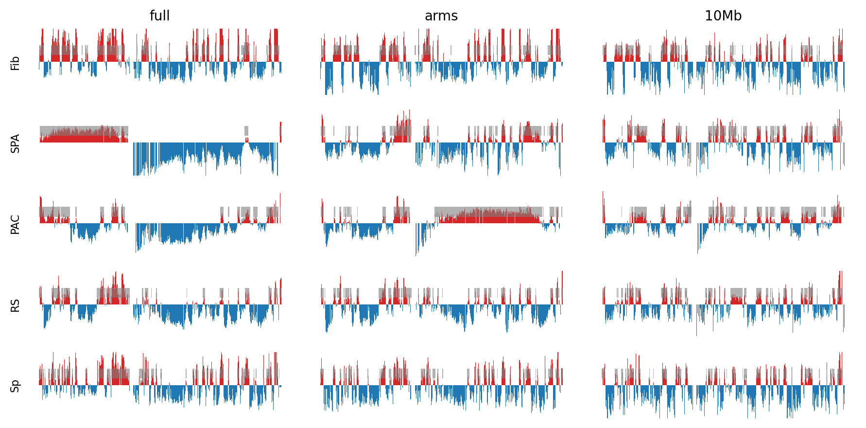
Plot matrices with compartments

import cooltools.lib.plotting
from matplotlib.colors import LogNorm
from mpl_toolkits.axes_grid1 import make_axes_locatable
from cooltools.lib.numutils import adaptive_coarsegrain, interp_nan

f, axs = plt.subplots(1,5,
    figsize=(25,10)
)

norm = LogNorm(vmax=0.1)

# Loop through the clrs and its matrix: plot the matrix on its axis
for i, (name, e1_dict) in enumerate(e1_values.items()):
    ax = axs[i]

    im = ax.matshow(
        clrs[name].matrix().fetch('chrX'),
        norm=norm,
        cmap='fall',
    );
    ax.set_xlim(0, nbins)
    ax.set_ylim(nbins, 0)

    divider = make_axes_locatable(ax)
    cax = divider.append_axes("right", size="2%", pad=0.05)
    plt.colorbar(im, cax=cax, label='corrected frequencies');
    ax.set_ylabel('chrX:100kb bins, #bin')
    ax.xaxis.set_visible(False)

    for j, (view, e1) in enumerate(e1_dict.items()):
        ax1 = divider.append_axes("top", size="10%", pad=0.1, sharex = ax)

        # ax1.plot(e1, label='E1')

        # Create stairs
        x = np.zeros(2*chrom_start.size)
        y = np.zeros(2*chrom_start.size)
        #smooth_y = np.zeros(2*chrom_start.size)
        x[0::2] = chrom_start/binsize
        x[1::2] = chrom_end/binsize
        y[0::2] = e1
        y[1::2] = e1
        # smooth_e1 = (lambda x: x.rolling(5, 1, center=True).sum())(pd.DataFrame(e1, columns=['value']))['value'].values
        # smooth_y[0::2] = smooth_e1
        # smooth_y[1::2] = smooth_e1


        ax1.fill_between(x, y, 0, where=(y > 0), color='tab:red', ec = 'None')
        ax1.fill_between(x, y, 0, where=(y < 0), color='tab:blue', ec = 'None')

        ax1.set_ylabel(view, rotation=-70)
        ax1.set_ylim(-0.8, 0.8)
        ax1.set_xticks([])

    ax1.set_title(abbr[name])

#    # Plot the sign changes on the matrix 
#     col = colors[i]
#     for i in np.where(np.diff( (pd.Series(e1)>0).astype(int)))[0]:
#         # Horisontal lines where E1 intersects 0
#         ax.plot([0,nbins],[i,i],col,lw=0.5)

#         # Vertical lines where E1 intersects 0
#         ax.plot([i,i],[0,nbins],col,lw=0.5)

# Now show the plot
f.set_layout_engine('compressed')
f.canvas.draw()
plt.show()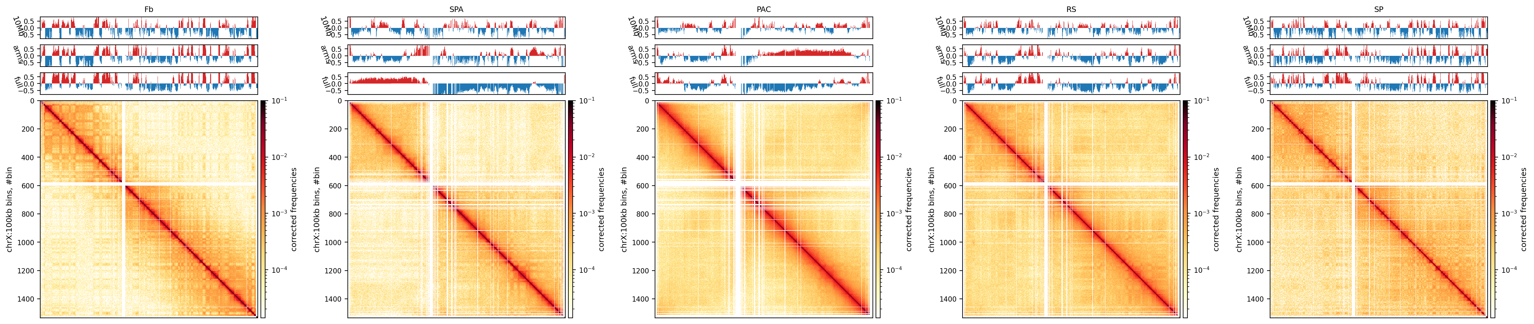

E1 eigenvector values for all merged samples at 500kb resolution for round spermatid, as well as the interaction matrix. E1 was restricted to top: Full-chromosome, middle: Chromosome-arms, bottom: 10Mb window.

import cooltools.lib.plotting
from matplotlib.colors import LogNorm
from mpl_toolkits.axes_grid1 import make_axes_locatable



clr = clrs['round_spermatid']
nbins = len(clr.bins().fetch('chrX'))

f, ax = plt.subplots(
    figsize=(3,3),
)

norm = LogNorm(vmax=0.1)

e1_dict = e1_values['round_spermatid']
e1_order = ['10Mb', 'arms', 'full']
e1_names_abbr = {'10Mb': '10Mb', 'arms': 'Arms', 'full': 'Full'}
colors = ['tab:red', 'tab:blue', 'tab:green']

# ### Coursegrain and interpolate (beautify)
# cg = adaptive_coarsegrain(clr.matrix(balance=True).fetch('chrX'),
#                           clr.matrix(balance=False).fetch('chrX'),
#                           cutoff=3, max_levels=8, )
# cgi = interp_nan(cg, method='nearest')

im = ax.matshow(
    clr.matrix().fetch('chrX'),
    norm=norm,
    cmap='fall',
);
plt.axis([0,nbins,nbins,0])


divider = make_axes_locatable(ax)
cax = divider.append_axes("right", size="4%", pad=0.05)
plt.colorbar(im, cax=cax, label='corrected frequencies');
ax.set_ylabel('Position (Mbp)')
ax.xaxis.set_visible(False)
yticks = np.linspace(0, nbins, 5, dtype=int)
yticklabels = yticks*100_000//1_000_000
ax.set_yticks(yticks)
ax.set_yticklabels(yticklabels)



for i, name in enumerate(e1_order):
    e1 = e1_dict[name]
    ax1 = divider.append_axes("top", size="10%", pad=0.05, sharex = ax)

    # Create stairs
    x = np.zeros(2*chrom_start.size)
    y = np.zeros(2*chrom_start.size)
    #smooth_y = np.zeros(2*chrom_start.size)
    x[0::2] = chrom_start/100_000
    x[1::2] = chrom_end/100_000
    y[0::2] = e1
    y[1::2] = e1
    # smooth_e1 = (lambda x: x.rolling(5, 1, center=True).sum())(pd.DataFrame(e1, columns=['value']))['value'].values
    # smooth_y[0::2] = smooth_e1
    # smooth_y[1::2] = smooth_e1


    ax1.fill_between(x, y, 0, where=(y > 0), color='tab:red', ec = 'None')
    ax1.fill_between(x, y, 0, where=(y < 0), color='tab:blue', ec = 'None')

    ax1.set_ylabel(e1_names_abbr[name], rotation=0, labelpad=5, ha='right', va='center')
    ax1.set_ylim(-0.8, 0.8)
    ax1.set_xticks([])
    ax1.set_yticks([])

    # if e1_names[i] == '10Mb':
    #     # Plot the sign changes on the matrix 
    #     col = 'k' #colors[i]
    #     for i in np.where(np.diff( (pd.Series(e1)>0).astype(int)))[0]:
    #         # Horisontal lines where E1 intersects 0
    #         ax.plot([0,nbins],[i,i],col,lw=0.5)

    #         # Vertical lines where E1 intersects 0
    #         ax.plot([i,i],[0,nbins],col,lw=0.2)

ax1.set_title('Round Spermatid: 100kb bins')
plt.tight_layout()
plt.show()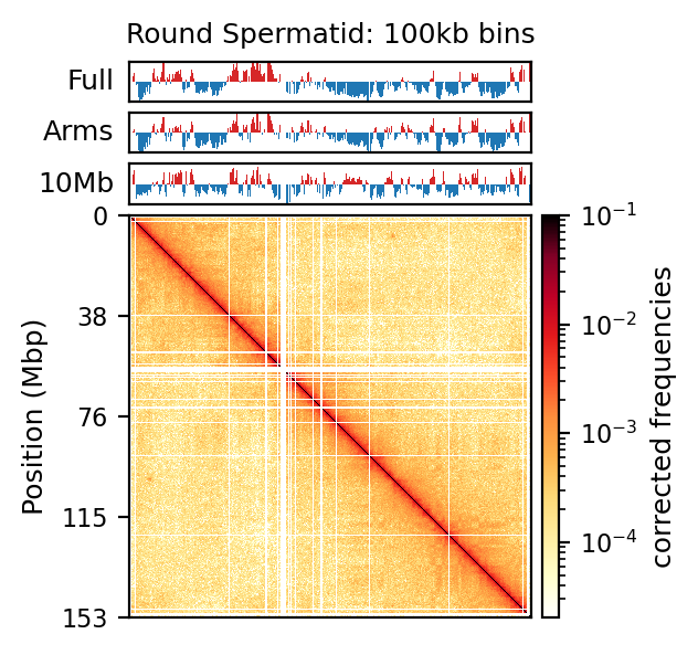

Figure 8.7: E1 eigenvector values for merged round spermatid samples at 500kb resolution, as well as the interaction matrix. E1 was restricted to either Full-chromosome (top), Chromosome-arms (middle), or 10Mb windows (bottom).

We continue plotting in the next notebook:

Link to notebook: Various Comparisons (07_various_plotting.ipynb)

Imakaev, Maxim, Geoffrey Fudenberg, Rachel Patton McCord, Natalia Naumova, Anton Goloborodko, Bryan R Lajoie, Job Dekker, and Leonid A Mirny. 2012. “Iterative Correction of Hi-C Data Reveals Hallmarks of Chromosome Organization.” Nature Methods 9 (10): 999–1003. https://doi.org/10.1038/nmeth.2148.

Wang, Yao, Hanben Wang, Yu Zhang, Zhenhai Du, Wei Si, Suixing Fan, Dongdong Qin, et al. 2019. “Reprogramming of Meiotic Chromatin Architecture During Spermatogenesis.” Molecular Cell 73 (3): 547–561.e6. https://doi.org/10.1016/j.molcel.2018.11.019.