# import standard python libraries
import numpy as np
import pandas as pd

# Import packages for working with cooler files and tools for plots
import cooler
import cooltools.lib.plotting
import cooltools
import seaborn as sns
from cooltools.lib.numutils import adaptive_coarsegrain, interp_nan
from matplotlib.colors import LogNorm
from mpl_toolkits.axes_grid1 import make_axes_locatable
Various Comparisons
Various plots using homemade plotting utility comparing different parameters and methods for the manuscript
Notes before we start
We want to create a plotting utility so we can easily plot and compare different matrices. We might move them to hicstuff.py for import, but as for now, they are defined only in this notebook.
Setup
Imports for plots etc
InlineBackend.rc
For consistent plots that fit with pdf manus.
import matplotlib.pyplot as plt

# Define my params:
## Params will comply with my desired layout for the Manuscript (PDF)

notebook_rcparams = {
    'font.size': 7,
    'axes.titlesize': 8,
    'axes.labelsize': 7,
    'xtick.labelsize': 6,
    'ytick.labelsize': 6,
    'figure.titlesize': 9,
    'figure.figsize': [6.0, 2.0],
    'figure.labelsize': 7,

}

# Apply config
%matplotlib inline
%config InlineBackend.figure_formats = ['retina']
%config InlineBackend.rc = notebook_rcparamsprint({key:plt.rcParams[key] for key in notebook_rcparams.keys()}){'font.size': 10.0, 'axes.titlesize': 'large', 'axes.labelsize': 'medium', 'xtick.labelsize': 'medium', 'ytick.labelsize': 'medium', 'figure.titlesize': 'large', 'figure.figsize': [6.4, 4.8], 'figure.labelsize': 'large'}## Apparently IPython needs this twice to understand??
import matplotlib.pyplot as plt
# Define my params:
## Params will comply with my desired layout for the Manuscript (PDF)
notebook_rcparams = {
'font.size': 7,
'axes.titlesize': 8,
'axes.labelsize': 7,
'xtick.labelsize': 6,
'ytick.labelsize': 6,
'figure.titlesize': 9,
'figure.figsize': [6.0, 2.0],
'figure.labelsize': 7,
}
# Apply config
%matplotlib inline
%config InlineBackend.figure_formats = ['retina']
%config InlineBackend.rc = notebook_rcparamsprint({key:plt.rcParams[key] for key in notebook_rcparams.keys()}){'font.size': 7.0, 'axes.titlesize': 8.0, 'axes.labelsize': 7.0, 'xtick.labelsize': 6.0, 'ytick.labelsize': 6.0, 'figure.titlesize': 9.0, 'figure.figsize': [6.0, 2.0], 'figure.labelsize': 7.0}Load all the coolers and eigenvectors
## Loading all coolers and their compartments
import glob
import os.path as op
import cooler

# Abbreviate the names (almost the same abbreviations as Wang et al. 2019)
names_abbr = {'fibroblast': 'Fib', 'spermatogonia': 'SPA', 'pachytene_spermatocyte': 'PAC', 'round_spermatid': 'RS', 'sperm': 'Sp'}

# Paths and resolutions
mcools = pd.Series(glob.glob("../steps/bwa/*/cool/*/*.mcool"))
res_100 = "::resolutions/100000"
res_500 = "::resolutions/500000"

# Create a DataFrame
clr_df = pd.DataFrame({
    'name': pd.concat([mcools.apply(lambda x: op.basename(op.dirname(x)))] * 3, ignore_index=True),
    'resolution': ['100'] * len(mcools) + ['ps500'] * len(mcools) + ['500'] * len(mcools),
    'mcool_path': pd.concat([mcools] * 3, ignore_index=True)
})

# Insert the 'sname' column (shortname/abbreviation)
clr_df['sname'] = clr_df['name'].apply(lambda x: names_abbr[x])

# Create the 'cooler_id' column
clr_df['cooler_id'] = clr_df.apply(
    lambda row: cooler.Cooler(
        row['mcool_path'] + (res_100 if row['resolution'] in ['100', 'ps500'] else res_500)
        ),
    axis=1
)

# Determine parsing run (dirname 3 levels up PE or recPE)
clr_df['run'] = clr_df['mcool_path'].apply(lambda x: 'recPE' if 'rec' in x else 'PE')

# Add the 'nbins' column
clr_df['nbins'] = clr_df['cooler_id'].apply(lambda x: len(x.bins().fetch('chrX')))

# Add the path to the compartments (../results/{compartments,rec_compartments})
# make a comp_dir dict
comp_dirs = {
    'PE': '../results/compartments/',
    'recPE': '../results/rec_compartments/'
}

clr_df['e1_dict'] = clr_df.apply(
    lambda row: {view: pd.read_csv(op.join(
        comp_dirs[row['run']], f"{row['name']}_e1_{row['resolution']}kb_{view}.csv"
        ))['e1']
        if row['resolution'] != 'ps500'
        else  pd.read_csv(op.join(
        comp_dirs[row['run']], f"{row['name']}_e1_100kb_{view}_smoothed.csv"
        ))['e1']
        for view in ['full', 'arms', '10Mb']},
    axis=1
)

# Now we have all the coolers and compartments ready for plotting (in semi-long format)
#clr_df
clr_df[['sname', 'resolution', 'nbins', 'run', 'e1_dict']].query('resolution == "ps500"')
#print(clr_df['e1_dict'].values)| sname | resolution | nbins | run | e1_dict | |
|---|---|---|---|---|---|
| 10 | PAC | ps500 | 1534 | recPE | {'full': [nan, nan, nan, nan, nan, nan, nan, n... |
| 11 | SPA | ps500 | 1534 | recPE | {'full': [nan, nan, nan, nan, nan, nan, nan, n... |
| 12 | Fib | ps500 | 1534 | recPE | {'full': [nan, nan, nan, nan, nan, -0.15077432... |
| 13 | RS | ps500 | 1534 | recPE | {'full': [nan, nan, nan, nan, nan, nan, nan, n... |
| 14 | Sp | ps500 | 1534 | recPE | {'full': [nan, nan, nan, nan, nan, -0.00698684... |
| 15 | RS | ps500 | 1534 | PE | {'full': [nan, nan, nan, nan, nan, -0.17383142... |
| 16 | SPA | ps500 | 1534 | PE | {'full': [nan, nan, nan, nan, nan, nan, nan, -... |
| 17 | Sp | ps500 | 1534 | PE | {'full': [nan, nan, nan, -0.102536873416233, -... |
| 18 | Fib | ps500 | 1534 | PE | {'full': [nan, nan, nan, -0.2342462339281897, ... |
| 19 | PAC | ps500 | 1534 | PE | {'full': [nan, nan, nan, nan, nan, 0.595328434... |
Load the genomic intervals
A-compartments
import pandas as pd
import os

# ECH regions and chromsizes
ech90 = pd.read_csv('../data/ech90_human_Mmul_10.csv').assign(length=lambda x: x.end - x.start)

chromsizes = (pd.read_csv(
    '../data/rheMac10.filtered.chrom.sizes',
    sep='\t',
    index_col='chrom',
    header=None,
    names=['chrom','size'])
.to_dict()['size']
)

# Directory containing your .csv files

comp_dirs = {
    'PE': '../results/compartments/',
    'recPE': '../results/rec_compartments/'
}

# Create a dictionary to store the comps
comps = {
    'PE': {},
    'recPE': {}
}

# Iterate over all .csv files in the directory
for run in comps.keys():
    comp_dir = comp_dirs[run]
    for filename in os.listdir(comp_dir):
        # We only want the .csv files and not e1 tracks
        if filename.endswith('.csv') and 'e1' not in filename:
            # Construct the full file path
            filepath = os.path.join(comp_dir, filename)

            # Load the CSV into a DataFrame
            # Use the filename (without extension) as the dictionary key
            key = filename.replace('_a_comp_coords_', '_')
            key = os.path.splitext(key)[0]
            comps[run][key] = pd.read_csv(filepath).assign(length=lambda x: x.end - x.start)

# The `comps` dictionary now contains the DataFrames
# Example usage:
comps['recPE']['round_spermatid_100kb_arms']| chrom | start | end | resolution | length | |
|---|---|---|---|---|---|
| 0 | chrX | 900000 | 1600000 | 100000 | 700000 |
| 1 | chrX | 1700000 | 2600000 | 100000 | 900000 |
| 2 | chrX | 2900000 | 3100000 | 100000 | 200000 |
| 3 | chrX | 3200000 | 3500000 | 100000 | 300000 |
| 4 | chrX | 6600000 | 6700000 | 100000 | 100000 |
| ... | ... | ... | ... | ... | ... |
| 72 | chrX | 145400000 | 147100000 | 100000 | 1700000 |
| 73 | chrX | 147300000 | 147400000 | 100000 | 100000 |
| 74 | chrX | 148800000 | 149100000 | 100000 | 300000 |
| 75 | chrX | 149300000 | 151200000 | 100000 | 1900000 |
| 76 | chrX | 152500000 | 153300000 | 100000 | 800000 |
77 rows × 5 columns
Edge intervals
import pandas as pd
import os

# Directory containing your .csv files
edge_dirs = {
    'PE': '../results/edges/',
    'recPE': '../results/rec_edges/'
}

edges = {
    'PE': {},
    'recPE': {}
}

# Iterate over all .csv files in the directories
for run in edges.keys():
    edge_dir = edge_dirs[run]
    for filename in os.listdir(edge_dir):
        if filename.endswith('.csv'):  # Check for .csv files
            # Construct the full file path
            filepath = os.path.join(edge_dir, filename)

            # Load the CSV into a DataFrame
            # Use the filename (without extension) as the dictionary key
            key = filename.replace('_edges', '')
            key = os.path.splitext(key)[0]
            edges[run][key] = pd.read_csv(filepath).assign(length=lambda x: x.end - x.start)

# The `edges` dictionary now contains the DataFrames
print(edges.keys())
display(edges['recPE']['fibroblast_100kb_10Mb'])

#ech90 = pd.read_csv('../data/ech90_human_Mmul_10.csv')
dict_keys(['PE', 'recPE'])| start | end | chrom | resolution | length | |
|---|---|---|---|---|---|
| 0 | 700000 | 900000 | chrX | 100000 | 200000 |
| 1 | 3300000 | 3500000 | chrX | 100000 | 200000 |
| 2 | 8200000 | 8400000 | chrX | 100000 | 200000 |
| 3 | 13300000 | 13500000 | chrX | 100000 | 200000 |
| 4 | 14900000 | 15100000 | chrX | 100000 | 200000 |
| ... | ... | ... | ... | ... | ... |
| 87 | 144400000 | 144800000 | chrX | 100000 | 400000 |
| 88 | 145400000 | 145600000 | chrX | 100000 | 200000 |
| 89 | 146700000 | 147100000 | chrX | 100000 | 400000 |
| 90 | 148800000 | 149000000 | chrX | 100000 | 200000 |
| 91 | 152100000 | 152300000 | chrX | 100000 | 200000 |
92 rows × 5 columns
Baboons
# Load baboons

import pandas as pd
from genominterv import interval_collapse

hama_panu3 = pd.read_csv('../data/lift/papanu4/high_hama_papanu4.bed', sep='\t', index_col=False, header=None, names=['group','chrom', 'start', 'end'])

olive_panu3 = pd.read_csv('../data/lift/papanu4/high_olive_papanu4.bed', sep='\t', index_col=False, header=None, names=['group','chrom', 'start', 'end'])

baboon_df = pd.read_csv('../results/high_baboon_rhemac10.bed', sep='\t', index_col=False, header=None, names=['chrom', 'start', 'end', 'group', 'score'])

high_hama_ucsc = (interval_collapse(baboon_df.query('group == "high_hama"')).
             assign(group = "high_hama").
             query('chrom == "chrX"')
             )
high_olive_ucsc = (interval_collapse(baboon_df.query('group == "high_olive"')).
              assign(group = "high_olive").
              query('chrom == "chrX"')
              )

high_hama = pd.read_csv('../data/lift/rheMac10/high_hama_rhemac10.bed', sep='\t', index_col=False, header=None, names=['group','chrom', 'start', 'end'])

high_olive = pd.read_csv('../data/lift/rheMac10/high_olive_rhemac10.bed', sep='\t', index_col=False, header=None, names=['group','chrom', 'start', 'end'])

baboon_dict = {"P.hama": high_hama, "P.anubis": high_olive}
Define a plotting utility for compartments and E1
This plots a group/subset of coolers and their respective E1 compartments.
# We can vary the number of subplots based on the number of coolers
# We can vary the number of views for each cooler
# We can define the region (tuple) of the chromosome to plot (default chrX)

def plot_grouped(
    group: pd.DataFrame,
    region: str = 'chrX', # or (chrom, start, end)
    include_compartments: bool = True,
    view_order: list[str] = ['10Mb', 'arms', 'full'],
    figsize: tuple[float, float] = (6, 6)
) -> None:

    group = group.reset_index(drop=True)

    # Define the number of subplots based on the number of coolers
    f, axs = plt.subplots(1,group.shape[0],
        figsize=figsize,
        sharex=True
    )

    # Logtransform the colorscale
    norm = LogNorm(vmax=0.1)

    # If there is only one cooler, axs is not a list, so we need to make it a list
    if not isinstance(axs, np.ndarray):
        axs = [axs]


    # Loop through the clrs and its matrix: plot the matrix on its axis
    for row in group.itertuples():
        ax = axs[row.Index]
        # Define the y-axis label
        title = f'{row.sname}{row.resolution}kb: {row.run}'
        ylab = f'{region}:{row.resolution}kb [Mb]'

        # Extract some variables
        e1_dict = {k: v for k, v in row.e1_dict.items() if k in view_order}
        chrom_start = row.cooler_id.bins().fetch(region)['start'].values
        chrom_end = row.cooler_id.bins().fetch(region)['end'].values

        im = ax.matshow(
            row.cooler_id.matrix().fetch(region),
            norm=norm,
            cmap='fall',
        );
        ax.set_xlim(0, row.nbins)
        ax.set_ylim(row.nbins, 0)
        ax.set_ylabel(ylab)
        ticks = np.linspace(0, row.nbins, 5)
        ax.set_yticks(ticks)
        ax.set_yticklabels([f'{x*row.cooler_id.binsize/1_000_000:.0f}' for x in ticks])
        ax.xaxis.set_visible(False)

        divider = make_axes_locatable(ax)
        cax = divider.append_axes("right", size="2%", pad=0.05)
        plt.colorbar(im, cax=cax, label='corrected frequencies');
        # Only show the colorbar on the last plot and ytitle on first plot
        if row.Index != group.shape[0] - 1:
            cax.set_visible(False)
        elif row.Index != 0:
            ax.set_ylabel('')

        # Skip the E1 plot when
        if not include_compartments:
            ax.set_title(title)
            continue

        for j, (view, e1) in enumerate(e1_dict.items()):
            ax1 = divider.append_axes("top", size="10%", pad=0.1, sharex = ax)

            # Create stairs
            x = np.zeros(2*chrom_start.size)
            y = np.zeros(2*chrom_start.size)
            x[0::2] = chrom_start/row.cooler_id.binsize
            x[1::2] = chrom_end/row.cooler_id.binsize
            y[0::2] = e1
            y[1::2] = e1

            ax1.fill_between(x, y, 0, where=(y > 0), color='tab:red', ec = 'None')
            ax1.fill_between(x, y, 0, where=(y < 0), color='tab:blue', ec = 'None')

            ax1.set_ylabel(view, rotation=0, ha='right', va='center')
            ax1.set_ylim(-0.8, 0.8)
            ax1.set_yticks([])
            ax1.set_xticks([])
            ax1.spines[:].set_visible(False)

        ax1.set_title(title)
    f.set_layout_engine('compressed')
    plt.show()
Plotting matrices separately
Plotting function that makes separate plots in stead of mpl.subplots. This makes it compatible with YAML header subfigures and layout options for embedding into Quarto
def plot_for_quarto(
    group: pd.DataFrame,
    region: str | tuple[str, int, int] = 'chrX',
    include_compartments: bool = True,
    view_order: list[str] = ['10Mb', 'arms', 'full'],
    figsize: tuple[float, float] = (6, 6),
    col_vmin: float = 1e-3,
    col_vmax: float = 0.1,
    save_png_name: str = None
) -> None:
    """
    Plot each cooler as a separate figure to allow Quarto YAML options for subfigure plots and captions.
    """
    group = group.reset_index(drop=True)

    # Scale figsize based on the number of coolers
    figsize = (figsize[0]/group.shape[0], figsize[1])

    # Set the region to a tuple if it is a string
    if isinstance(region, str):
        region = (region, 0, group.iloc[0].cooler_id.chromsizes[region])

    # Define start and end for the matrix plot
    start, end = region[1], region[2]

    # Loop through each cooler (row) in the DataFrame
    for row in group.itertuples():
        # Create a new figure for each cooler
        # Scale figsize
        fig, ax = plt.subplots(figsize=figsize)

        # Logtransform the colorscale
        norm = LogNorm(vmin=col_vmin,vmax=col_vmax)

        # Define the y-axis label
        # title = f'{row.sname}{row.resolution}kb: {row.run}'
        ylab = f'{row.resolution}kb'

        # Extract some variables
        e1_dict = {k: row.e1_dict[k] for k in view_order}
        chrom_start = row.cooler_id.bins().fetch(region)['start'].values
        chrom_end = row.cooler_id.bins().fetch(region)['end'].values
        nbins = chrom_start.size # != row.nbins when subsetting chr
        binsize = row.cooler_id.binsize # is used several times

        # Plot the Hi-C matrix
        im = ax.matshow(
            row.cooler_id.matrix().fetch(region),
            norm=norm,
            cmap='fall',
            extent=(0, nbins, nbins, 0)
        )
        ax.set_xlim(0, nbins)
        ax.set_ylim(nbins, 0)
        ax.set_ylabel(ylab)
        ticks = np.linspace(0, nbins, 5)
        ax.set_yticks(ticks)
        ax.set_yticklabels([f'{(start/binsize+x)*binsize/1_000_000:.0f}' for x in ticks])
        ax.xaxis.set_visible(False)

        # Add a colorbar
        divider = make_axes_locatable(ax)
        cax = divider.append_axes("right", size="2%", pad=0.05)
        plt.colorbar(im, cax=cax, label='corrected frequencies')

        # Skip E1 plot if not including compartments
        if include_compartments:
            for view, e1 in e1_dict.items():
                # subset the e1 to region (chrX:start-end)/binsize
                start_bin = int(chrom_start[0]/binsize)
                end_bin = int(chrom_start[-1]/binsize)
                e1 = e1.iloc[start_bin:end_bin+1].reset_index(drop=True)
                ax1 = divider.append_axes("top", size="10%", pad=0.05, sharex=ax)

                # Create stairs for E1 values
                x = np.zeros(2 * chrom_start.size)
                y = np.zeros(2 * chrom_start.size)
                x[0::2] = np.arange(chrom_start.size)
                x[1::2] = np.arange(chrom_start.size)
                y[0::2] = e1
                y[1::2] = e1

                ax1.fill_between(x, y, 0, where=(y > 0), color='tab:red', ec='None')
                ax1.fill_between(x, y, 0, where=(y < 0), color='tab:blue', ec='None')

                if len(e1_dict) > 1:
                    ax1.set_ylabel(view, rotation=0, ha='right', va='center', fontsize=7)
                else:
                    ax1.set_ylabel('E1', rotation=0, ha='right', va='center', fontsize=7)

                ax1.set_ylim(-0.8, 0.8)
                ax1.set_yticks([])
                ax1.set_xticks([])
                ax1.spines[:].set_visible(False)

        # # Set the figure title
            # ax1.set_title(title)

        fig.tight_layout()

        if save_png_name:
            plt.savefig(save_png_name, dpi=320)

        # Display the figure for Quarto to capture
        plt.show()
Plot intervals
Plot genomic intervals as tracks (up to 3)
import matplotlib.pyplot as plt
import numpy as np
import pandas as pd
from matplotlib.patches import Rectangle
from mpl_toolkits.axes_grid1 import make_axes_locatable
from genominterv import interval_intersect


def plot_regions(query=None, annot=None, intersect=None,
                 track_titles=['query', 'annot', 'intersect'],
                 figsize=(10, 1),
                 title='chrom',
                 alpha=0.8, lw=0):
    chrom = annot['chrom'].unique()[0]
    chromsizes = pd.read_csv('../data/rheMac10.filtered.chrom.sizes', sep='\t', header=None, names=['chrom', 'size'])

    base_size = chromsizes[chromsizes['chrom'] == chrom]['size'].values[0]
    annot_size = annot['end'].max()
    query_size = query['end'].max()
    chromsize = max(base_size, annot_size, query_size)


    if title == 'chrom':
        title = chrom


    # Define the plot size

    f, ax = plt.subplots(figsize=figsize, sharex=True)

    ax.spines[:].set_visible(False)

    # Plot the annot
    # Iterate over each interval in the DataFrame
    for start, end in zip(annot['start'], annot['end']):
        rect = Rectangle((start, 0.1), width=end-start, height=0.9, color='tab:red', linewidth=lw, alpha=alpha)
        ax.add_patch(rect)
        ax.spines['bottom'].set_visible(True)
        ax.set_ylabel(track_titles[1], rotation=0, labelpad=10, ha='right', va='center')


    divider = make_axes_locatable(ax)

    if query is not None:
        qax = divider.append_axes("top", size="100%", pad=0.05, sharex=ax)
        qax.xaxis.set_visible(False)
        # Plot the query
        for start, end in zip(query['start'], query['end']):
            rect = Rectangle((start, 0.1), width=end-start, height=0.9, color='tab:blue', linewidth=lw, alpha=alpha)
            qax.add_patch(rect)
            qax.spines[:].set_visible(False)
            qax.set_yticks([])
            qax.set_title(title, loc='left')
            qax.set_ylabel(track_titles[0], rotation=0, labelpad=10, ha='right', va='center')

    if intersect is not None:
        iax = divider.append_axes("bottom", size="100%", pad=0.05, sharex=ax)
        # Invisible x-axis for 'annot' (intersect ie below)
        ax.xaxis.set_visible(False)
        # Plot the intersect
        for start, end in zip(intersect['start'], intersect['end']):
            rect = Rectangle((start, 0.1), width=end-start, height=0.9, color='tab:green', linewidth=lw, alpha=alpha)
            iax.add_patch(rect)
            iax.spines[:].set_visible(False)
            iax.set_yticks([])
            ax.spines['bottom'].set_visible(False)
            iax.spines['bottom'].set_visible(True)
            iax.set_ylabel(track_titles[2], rotation=0, labelpad=10, ha='right', va='center')


    ax.set_yticks([])
    ax.set_xlim(0, chromsize)
    ticks = np.linspace(0, chromsize, num=5)
    ax.set_xticks(ticks)
    ax.set_xticklabels([f'{int(t/1e6)} Mbp' for t in ticks])
    f.tight_layout()
    plt.show()
    #plt.tight_layout()
Make edges
def make_edges(df, resolution):
    start_edge = pd.DataFrame({
        'chrom': df['chrom'],
        'start': df.apply(lambda x: max(x['start'] - resolution, 0), axis=1),
        'end': df['start']+1*resolution,
        'resolution': resolution,
    })
    end_edge = pd.DataFrame({
        'chrom': df['chrom'],
        'start': df['end']-1*resolution,
        'end': df.apply(lambda x: min(x['end'] + resolution, chromsizes['chrX']), axis=1),
        'resolution': resolution,
    })

    return interval_collapse(pd.concat([start_edge, end_edge]).sort_values(['chrom', 'start', 'end'])).assign(resolution=resolution)
Svedig tabel
all_tests = pd.read_csv('../results/all_tests.csv', index_col=0)

def svedig_tabel(orig_df, index, columns, values,
                 cmap='Reds', col_order=None, col_snames=None):

    """
    Creates a styled pivot table from a DataFrame, filtering by significance,
    applying a log transformation, and adding visual styling.

    Parameters:
    ----------
    orig_df : pd.DataFrame
        The original DataFrame containing data to be processed.
    index : str
        Column name to use as the row index in the pivot table.
    columns : str
        Column name to use as the column headers in the pivot table.
    values : str
        Column name whose values populate the pivot table cells.
    cmap : str, optional
        Colormap to use for the background gradient styling (default is 'Reds').

    Returns:
    -------
    pd.io.formats.style.Styler
        A styled DataFrame object with the pivot table, including gradient-based
        cell coloring, transparent NaN values, formatted numbers, and table styles.
    """

    df = (orig_df
     .assign(log10p=np.log10(all_tests.p))
     .loc[(all_tests.p < 0.05)]
     .pivot(index=index, columns=columns, values=values)
    )
    if col_order:
        col_bool = [x in df.columns for x in col_order]
        col_order = [x for x in col_order if x in df.columns]
        df = df[col_order]
    if col_snames:
        col_snames = [col_snames[i] for i,x in enumerate(col_bool) if x]
        df = df.rename(columns = {x:col_snames[i] for i,x in enumerate(df.columns.tolist())})
    else:
        df = df.rename(columns = {x:x.replace('_', '<br>') for x in df.columns.tolist()})
    df = (df.style
     .background_gradient(subset=df.columns, axis=None, cmap=cmap, vmin=0)
     .map(lambda x: 'color: transparent; background-color: transparent' if np.isnan(x) else '')
     .format('{:.3f}')
     .set_table_styles(
                {c: [{'selector': '',
                      'props': [('min-width', '20px')],
                     }] for c in df.columns}, overwrite=False
     )
    )
return dfprint("That should be all the setup :-)")That should be all the setup :-)Matrices / E1
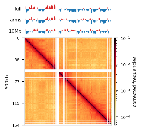
E1: RS100/500
# Compare the compartments of the round_spermatid, 500kb, all views
res = ['100', '500']
name = ['round_spermatid']
run = ['recPE']

group = clr_df.query('name in @name and resolution in @res and run in @run')
plot_for_quarto(group)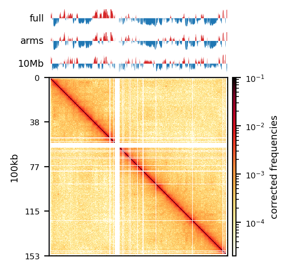
PE vs recPE (RS100kb)
# Compare PE and recPE compartments for round_spermatid, 100kb

group = clr_df.query('resolution == "100" and name == "round_spermatid"')

plot_grouped(group, figsize=(6, 6))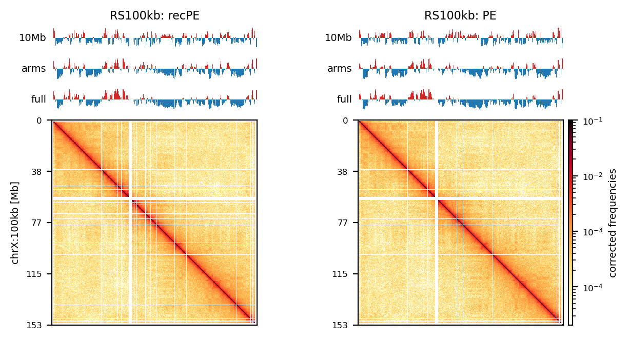
df = clr_df.query('resolution == "500" and name == "round_spermatid" and run == "PE"')

plot_grouped(df, include_compartments=False, figsize=(3, 3))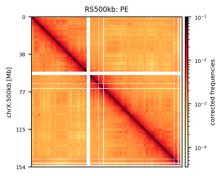
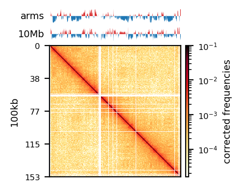
PE vs. recPE: RS100kb
df = clr_df.query('resolution == "100" and name == "round_spermatid"')
# Check the order of the group
#print(df[['name', 'resolution', 'run']].reset_index(drop=True))
plot_for_quarto(df, view_order=['10Mb','arms'], figsize=(5, 5))
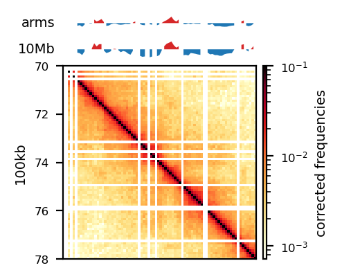
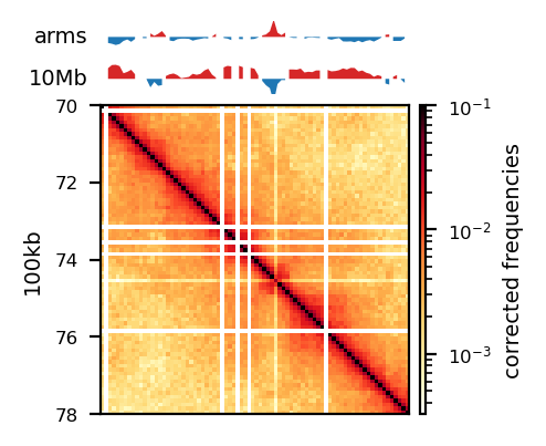
start, end = 70_000_000, 78_000_000
region = ('chrX', start, end)
plot_for_quarto(df, region=region, include_compartments=True, view_order=['10Mb','arms'], figsize=(5, 5))

5unique: chrX:start-end
mask: chrX:start-end
5unique: chrX:70Mb-78Mb
mask: chrX:70Mb-78Mb
Intervals
PE/recPE compare compartments (100kb)
from genominterv import interval_diff
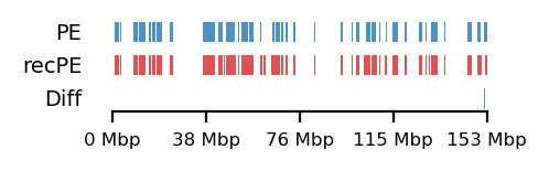
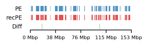
### Plot the intervals and the diff between ###
# Round Spermatid arms
query = comps['PE']['round_spermatid_100kb_arms']
annot = comps['recPE']['round_spermatid_100kb_arms']
plot_regions(query=query, annot=annot,
intersect=interval_diff(query, annot),
track_titles=['PE', 'recPE', 'Diff'],
figsize=(2.5, 0.8),
title=None)
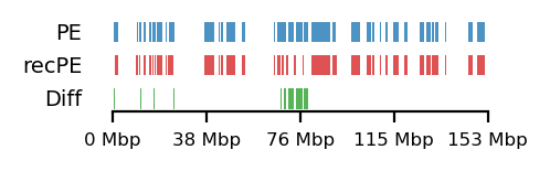
# Fibroblast arms
query = comps['PE']['fibroblast_100kb_arms']
annot = comps['recPE']['fibroblast_100kb_arms']
plot_regions(query=query, annot=annot,
intersect=interval_diff(query, annot),
track_titles=['PE', 'recPE', 'Diff'],
figsize=(2.5, 0.8),
title=None)
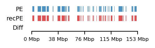
# Round Spermatid 10Mb
query = comps['PE']['round_spermatid_100kb_10Mb']
annot = comps['recPE']['round_spermatid_100kb_10Mb']
plot_regions(query=query, annot=annot,
intersect=interval_diff(query, annot),
track_titles=['PE', 'recPE', 'Diff'],
figsize=(2.5, 0.8),
title=None)
# Fibroblast 10Mb
query = comps['PE']['fibroblast_100kb_10Mb']
annot = comps['recPE']['fibroblast_100kb_10Mb']
plot_regions(query=query, annot=annot,
intersect=interval_diff(query, annot),
track_titles=['PE', 'recPE', 'Diff'],
figsize=(2.5, .8),
title=None)
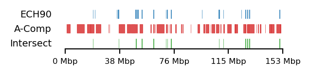
from genominterv import interval_intersect
query = ech90
fb_ann_comp = comps['recPE']['fibroblast_100kb_arms']
rs_ann_comp = comps['recPE']['round_spermatid_100kb_arms']
fb_ann_edge = edges['recPE']['fibroblast_100kb_arms']
rs_ann_edge = edges['recPE']['round_spermatid_100kb_arms']
size=(3.2, 0.8)
# Fib and RS compartments
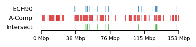
plot_regions(query=query, annot=fb_ann_comp,
intersect=interval_intersect(query, fb_ann_comp),
track_titles=['ECH90', 'A-Comp', 'Intersect'],
figsize=size,
title=None,
lw=0.3)
plot_regions(query=query, annot=rs_ann_comp,
intersect=interval_intersect(query, rs_ann_comp),
track_titles=['ECH90', 'A-Comp', 'Intersect'],
figsize=size,
title=None,
lw=0.3)
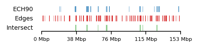
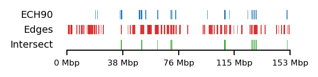
# Fib and RS edges
plot_regions(query=query, annot=fb_ann_edge,
intersect=interval_intersect(query, fb_ann_edge),
track_titles=['ECH90', 'Edges', 'Intersect'],
figsize=size,
title=None,
lw=0.3, alpha=1)
plot_regions(query=query, annot=rs_ann_edge,
intersect=interval_intersect(query, rs_ann_edge),
track_titles=['ECH90', 'Edges', 'Intersect'],
figsize=size,
title=None,
lw=0.3, alpha=1)
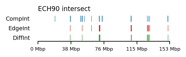
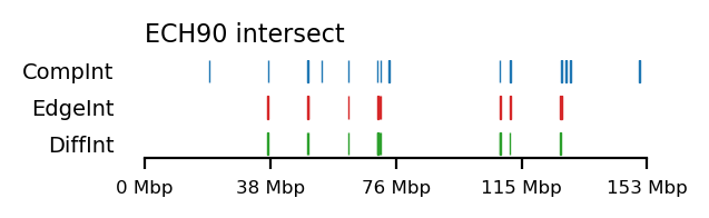
Visualize ECH enrichment
from genominterv import interval_diff, interval_intersect, interval_union

complist = [comps['recPE']['round_spermatid_100kb_arms'],
            comps['recPE']['fibroblast_100kb_arms']]
edgelist = [edges['recPE']['round_spermatid_100kb_arms'],
            edges['recPE']['fibroblast_100kb_arms']]

for comp, edge in zip(complist, edgelist):
    int_comp = interval_intersect(ech90, comp)
    int_edge = interval_intersect(ech90, edge)

    diff_int_compedge = interval_diff(int_edge, int_comp)
    plot_regions(int_comp, int_edge, diff_int_compedge,
                track_titles=['CompInt', 'EdgeInt', 'DiffInt'],
                title="ECH90 intersect",
                figsize=(3.2, 1),
                alpha=1, lw=0.5)
All 3 sets
plot_regions(ech90, high_olive, high_hama,
             track_titles=['ECH90', r"$\it{P.anubis}$", r"$\it{P.hama}$"],
             figsize=(5, 0.8),
             title=None,
             lw=0.5, alpha=0.8)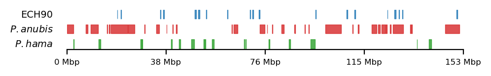
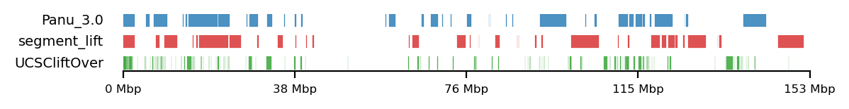
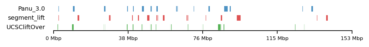
LiftOver comparison
track0 = [olive_panu3, hama_panu3]
track1 = [high_olive, high_hama]
track2 = [high_olive_ucsc, high_hama_ucsc]

for t0,t1,t2 in zip(track0, track1, track2):
    plot_regions(t0,t1,t2,
                track_titles=['Panu_3.0', 'segment_lift','UCSCliftOver'],
    #            title='High Olive Ancestry Intervals',
                title=None,
                figsize=(6, 0.8),
                alpha=0.8, lw=0.1)
Baboon-rs100-intersect
# Plot

size = (3.2, 0.8)
edge_rs = edges['recPE']['round_spermatid_100kb_arms']

for name,group in baboon_dict.items():
    plot_regions(query=edge_rs, annot=group,
                 intersect=interval_intersect(edge_rs, group),
                 #intersect=ech90,
                 track_titles=['RS100', fr"$\it{{{name}}}$", 'Intersect'],
                 figsize=size,
                 title=None,
                 lw=0.3, alpha=0.9)

edge_rs = edges['recPE']['round_spermatid_100kb_10Mb']

for name,group in baboon_dict.items():
    plot_regions(query=edge_rs, annot=group,
                 intersect=interval_intersect(edge_rs, group),
                 #intersect=ech90,
                 track_titles=['RS100', fr"$\it{{{name}}}$", 'Intersect'],
                 figsize=size,
                 title=None,
                 lw=0.2, alpha=1)
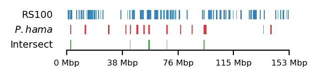
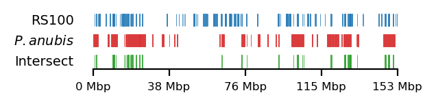
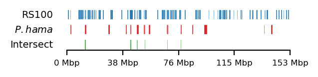

Table: Test 1bp limits
all_tests.head() #.query('query == "hama_edge_1bp"')| tissue | pc_scale | query | annot | test | value | p | -log10p | |
|---|---|---|---|---|---|---|---|---|
| 0 | fibroblast | arms | ECH90 | comp_edge_1bp | jaccard | 0.000002 | 0.01656 | 1.780940 |
| 1 | fibroblast | arms | hama_edge_1bp | comp_edge_1bp | proximity | 0.221717 | 0.88421 | 0.053445 |
| 2 | fibroblast | arms | olive_edge_1bp | comp_edge_1bp | proximity | 0.243643 | 0.67235 | 0.172405 |
| 3 | fibroblast | arms | olivehama_edge_1bp | comp_edge_1bp | proximity | 0.243643 | 0.74099 | 0.130188 |
| 4 | fibroblast | 10Mb | ECH90 | comp_edge_1bp | jaccard | 0.080105 | 0.02146 | 1.668370 |
tissue_order = ['fibroblast', 'spermatogonia', 'pachytene_spermatocyte', 'round_spermatid', 'sperm']
tissue_sname = ['Fb', 'Spa', 'Pac', 'RS', 'Sperm']


t0 = (svedig_tabel(all_tests
                   .map(lambda x: x.replace('_edge_1bp', '') if isinstance(x, str) else x)
                   .rename(columns={'pc_scale': 'viewframe'}),
             index=['viewframe', 'test','query'],
             columns=["tissue"],
             col_order = tissue_order,
             col_snames = tissue_sname,
             values='p',
             cmap='Reds_r')
)

t1 = (svedig_tabel(
    all_tests
    .map(lambda x: x.replace('_edge_1bp', '') if isinstance(x, str) else x)
    .query('pc_scale == "arms"'),
    index=['test','query'],
    columns=["tissue"],
    col_order = tissue_order,
    col_snames = tissue_sname,
    values='p',
    cmap='Reds_r')
#.relabel_index(labels=[lbl for lbl in tissue_sname if lbl in t1.columns], axis=1)
)

t2 = (svedig_tabel(all_tests
                   .map(lambda x: x.replace('_edge_1bp', '') if isinstance(x, str) else x)
                   .query('pc_scale == "10Mb"'),
             index=['test','query'],
             columns=["tissue"],
             col_order = tissue_order,
             col_snames = tissue_sname,
             values='p',
             cmap='Reds_r')
)


display(t0)| tissue | Fb | Spa | Pac | RS | Sperm | ||
|---|---|---|---|---|---|---|---|
| viewframe | test | query | |||||
| 10Mb | jaccard | ECH90 | 0.021 | 0.006 | nan | nan | 0.048 |
| proximity | olive | nan | nan | nan | nan | 0.016 | |
| olivehama | nan | 0.019 | 0.012 | nan | 0.001 | ||
| arms | jaccard | ECH90 | 0.017 | 0.006 | 0.005 | 0.028 | nan |
| proximity | olivehama | nan | nan | 0.036 | nan | nan |
tissue_order = ['fibroblast', 'spermatogonia', 'pachytene_spermatocyte', 'round_spermatid', 'sperm']
tissue_sname = ['Fb', 'Spa', 'Pac', 'RS', 'Sperm']


df = (all_tests
      .map(lambda x: x.replace('_edge_1bp', '_1bp') if isinstance(x, str) else x)
      .assign(log10p=np.log10(all_tests.p))
      .loc[(all_tests.p < 0.05)]
      .pivot(index=['pc_scale', 'query', 'test' ], columns=["tissue"], values="p").
      filter(tissue_order)
)

df = df.rename(columns = {x:tissue_sname[i] for i,x in enumerate(df.columns.tolist())})
df.columns.name = None
df = df.reset_index().fillna('-')
df = df.rename(columns={'pc_scale': 'View', 'query': 'Query', 'test': 'Test'})
df.style.hide(axis='index')| View | Query | Test | Fb | Spa | Pac | RS | Sperm |
|---|---|---|---|---|---|---|---|
| 10Mb | ECH90 | jaccard | 0.021460 | 0.006110 | - | - | 0.047500 |
| 10Mb | olive_1bp | proximity | - | - | - | - | 0.016140 |
| 10Mb | olivehama_1bp | proximity | - | 0.018790 | 0.012300 | - | 0.001280 |
| arms | ECH90 | jaccard | 0.016560 | 0.006120 | 0.005340 | 0.027690 | - |
| arms | olivehama_1bp | proximity | - | - | 0.035640 | - | - |
Figures for the defence
%config InlineBackend.figure_formats = ['retina']group = clr_df.query('name == "sperm" and resolution == "500" and run == "recPE"')
slide_path = "../slides/images/hic-example.png"
plot_for_quarto(group, view_order=['10Mb'],
col_vmin=1e-4, col_vmax=0.5,
save_png_name=slide_path)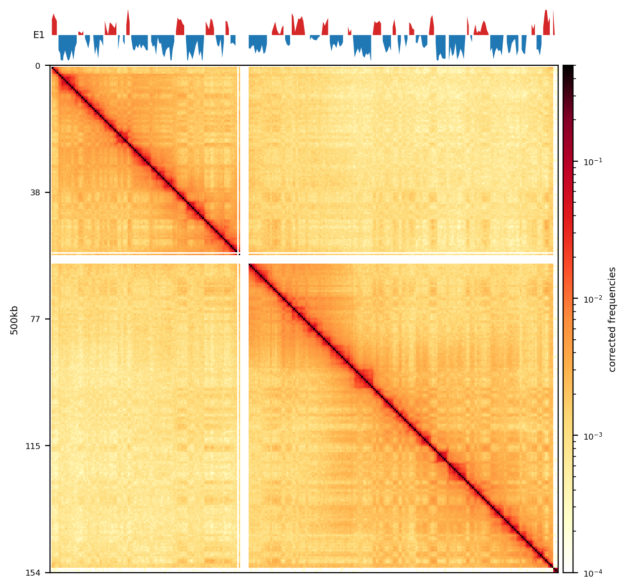
Introduce selected regions
plot_regions(ech90, high_olive, high_hama,
             track_titles=['ECH90', r"$\it{P.anubis}$", r"$\it{P.hama}$"],
             figsize=(10, 1.5),
             title=None,
             lw=0.5, alpha=0.8)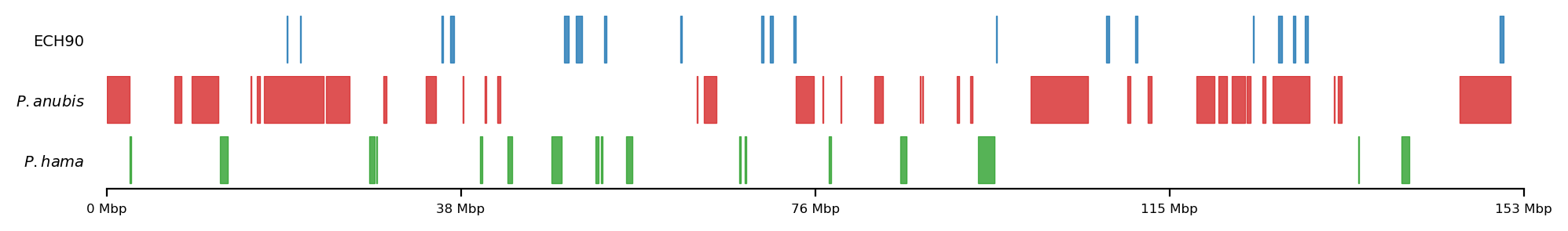
Compare liftover
from genominterv import interval_union

track0 = [olive_panu3, hama_panu3]
track1 = [high_olive, high_hama]
track2 = [high_olive_ucsc, high_hama_ucsc]

track0 = [interval_union(olive_panu3, hama_panu3)]
track1 = [interval_union(high_olive, high_hama)]
track2 = [interval_union(high_olive_ucsc, high_hama_ucsc)]

for t0,t1,t2 in zip(track0, track1, track2):
    plot_regions(t0,t1,t2,
                track_titles=['Panu_3.0', 'segment_lift','UCSCliftOver'],
    #            title='Baboon Intervals',
                title=None,
                figsize=(10, 1.5),
                alpha=0.8, lw=0.2)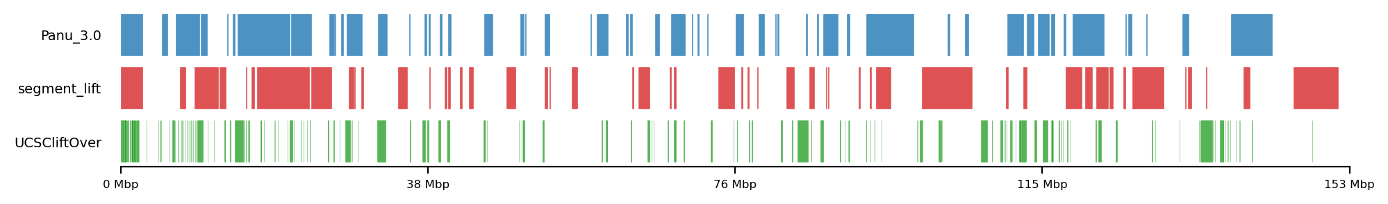
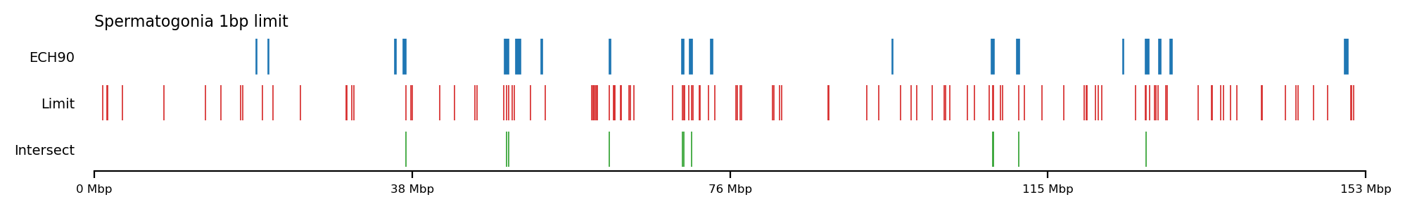
ECH S100 limit intersect
annot = make_edges(comps['recPE']['fibroblast_100kb_arms'], 2)
query = ech90

plot_regions(query=query, annot=annot,
             intersect=interval_intersect(query, annot),
             track_titles=['ECH90', 'Limit', 'Intersect'],
             figsize=(10, 1.5),
             title="Spermatogonia 1bp limit",
             lw=0.6, alpha=1)
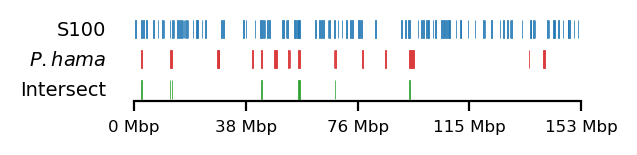
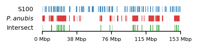
# Plot
size = (3.2, 0.8)
edge_rs = edges['recPE']['sperm_100kb_arms']
for name,group in baboon_dict.items():
plot_regions(query=edge_rs, annot=group,
intersect=interval_intersect(edge_rs, group),
#intersect=ech90,
track_titles=['S100', fr"$\it{{{name}}}$", 'Intersect'],
figsize=size,
title=None,
lw=0.3, alpha=0.9)
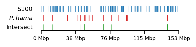
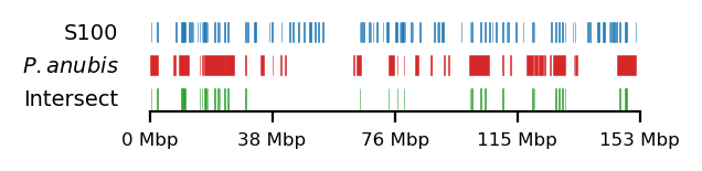
edge_rs = edges['recPE']['sperm_100kb_10Mb']
for name,group in baboon_dict.items():
plot_regions(query=edge_rs, annot=group,
intersect=interval_intersect(edge_rs, group),
#intersect=ech90,
track_titles=['S100', fr"$\it{{{name}}}$", 'Intersect'],
figsize=size,
title=None,
lw=0.2, alpha=1)