Discrete distributions

from phasic import Graph, with_ipv
import sys
import numpy as np
import pandas as pd
import matplotlib.pyplot as plt
from matplotlib.colors import LogNorm
import seaborn as sns
import vscodenb
sns.set_palette('tab10')
np.random.seed(42)

Consider this simple graph representing an exponential distribution. If you must, you can make it the coalescence time of two lineages in very small population:

def exponential(state):
    transitions = []               # List for transitions from state
    if state[0] < 2:               # Control transitions allowed
        child = state.copy()       # Make a copy to modify
        child[0] += 1              # Make the child state
        trans = [child, 2.0]       # Pair the child with a transition rate
        transitions.append(trans)  # Append transition 
    return transitions

graph = Graph(exponential, ipv=[1])
graph.plot()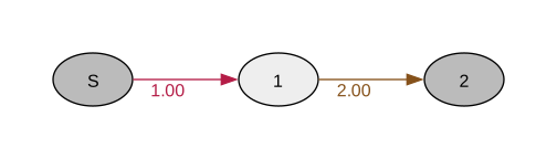

def exponential(rate):
    graph = Graph(1)
    vertex = graph.find_or_create_vertex([2])
    graph.starting_vertex().add_edge(vertex, 1)
    abs_vertex = graph.find_or_create_vertex([1])
    vertex.add_edge(abs_vertex, rate)
    return graph

graph = exponential(0.4)
graph.plot()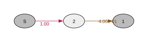

rate = 0.4
x = np.arange(0, 10, 0.01)
graph = exponential(rate)
plt.plot(x, graph.cdf(x))
plt.show()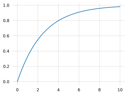

Discrete phase-type distributions represent the the number of jumps in a Markov Chain before absorption. We can discretize our graph it to get a geometric distribution:

graph = exponential(0.4)
print(f'is discrete: {graph.is_discrete}')
graph = graph.discretize(1-rate)
print(f'is discrete: {graph.is_discrete}')
graph.plot()

is discrete: False
is discrete: True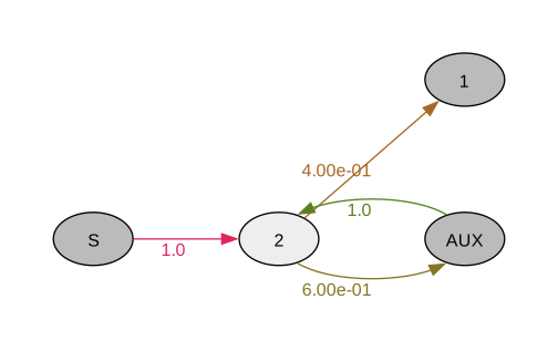

The discretize method returns a new graph, by connecting each non-absorbing vertex in the graph to an auxiliary vertex with a specified rate. Each AUX vertex connects to its parent with rate 1. Once AUX vertices are added, the graph is normalized so the sum of edge weights sum to 1 for each vertex. The returned graph has a .rewards attribute containing the indices of the added AUX vertices:

graph.rewards

array([0, 0, 0, 1])

The is_discrete attribute is set to True.

graph.is_discrete

True

Tip

NB: if you manually construct a discrete grap, you need to either set graph.is_discrete = True.

x = np.arange(10)
cdf = graph.reward_transform(graph.rewards).cdf(x)
plt.hlines(y=cdf, xmin=x, xmax=x+1, zorder=1, color='lightblue')
plt.scatter(x, cdf, s=18)
plt.show()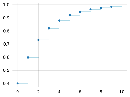

Figure 2: Continuous (exponential) distribution

To model discrete mutations with rate 0.1 along branches of the coalescent tree, we just discretize the continuous coalescent.

nr_samples = 4

@with_ipv([nr_samples]+[0]*(nr_samples-1))
def coalescent(state):
    transitions = []
    for i in range(state.size):
        for j in range(i, state.size):      
            same = int(i == j)
            if same and state[i] < 2:
                continue
            if not same and (state[i] < 1 or state[j] < 1):
                continue 
            new = state.copy()
            new[i] -= 1
            new[j] -= 1
            new[i+j+1] += 1
            transitions.append((new, state[i]*(state[j]-same)/(1+same)))

    return transitions

graph = Graph(coalescent)
assert not graph.parameterized()
graph.plot()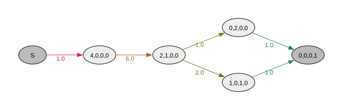

As alternative to a fixed rate, discretize also accepts a callable that maps each state vector to a rate. In this case we want the rate to scale with the number of live lineages on which mutations can happen:

mutation_rate = 0.3

# def mutation(state:np.ndarray, mutation_rate:float):
def mutation_callback(state):
    nr_lineages = sum(state)
    return nr_lineages * mutation_rate

mutation_graph = graph.discretize(rate=mutation_callback)
aux_rewards = mutation_graph.rewards

The auxiliary nodes added have dummy states with all zeros and are labelled as “AUX” vertices when the graph is plotted:

mutation_graph.plot(nodesep=0.5, size=(6, 4))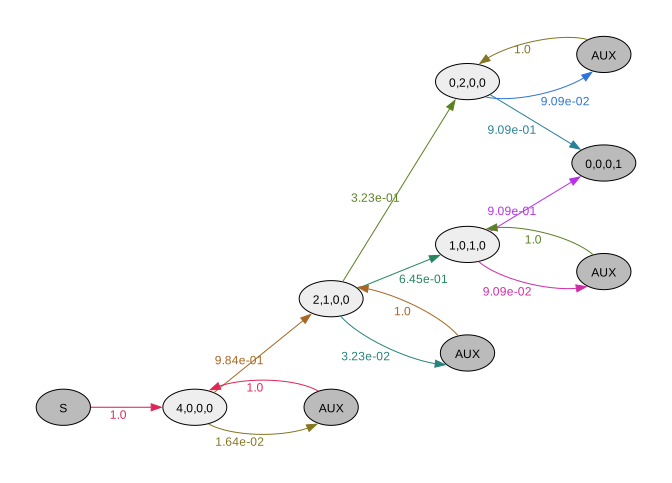

To compute the expected number of mutations, we apply rewards such that each AUX vertex get a reward of 1 and all other states a reward of 0. This is already encoded in the rewards attribute fo the discretized graph:

mutation_graph.expectation(mutation_graph.rewards)

1.0999999999999999

We can verify that the expected number of mutations correspond to the total branch length scaled with the mutation rate:

graph = Graph(coalescent)
tot_brlen = graph.expectation(graph.states().T.sum(axis=0))
tot_brlen * mutation_rate

1.0999999999999999

Or compare it to emprical mean of samples from the models

samples = mutation_graph.sample(10000, rewards=aux_rewards)
samples.mean().item()

1.1249

_rewards = graph.states().T
_rewards = _rewards[:-1].sum(axis=0)
samples = graph.sample(10000, rewards=_rewards)
samples.mean().item() * mutation_rate

1.1131379232943204

If we reward transform the graph, we can find the distribution function for the the total number of mutations:

rev_trans_mutation_graph  = mutation_graph.reward_transform_discrete(aux_rewards)
rev_trans_mutation_graph.plot(nodesep=0.4, size=(6, 4))

Notice that with this reward transformation the graph is no longer sparse, as all paths through the graph are represented.

x = np.arange(20)
pmf = rev_trans_mutation_graph.pdf(x)
cdf = rev_trans_mutation_graph.cdf(x)

fig, (ax1, ax2) = plt.subplots(1, 2, figsize=(8, 3))
ax1.bar(x, pmf)
ax1.set_title("PDF")
ax1.set_xlabel('Total number of mutations')
left, right = x, np.arange(1, x.size+1, 1)
ax2.hlines(y=cdf, xmin=left, xmax=right, zorder=1)
ax2.scatter(left, cdf, s=15, zorder=2)
ax2.set_title("CDF")
ax2.set_xlabel('Total number of mutations')
ax2.axhline(y=1-mutation_graph.defect(), ls='--', lw=0.5, c='k', label='1 - defect')
plt.legend() ;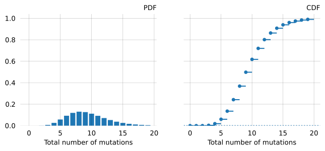

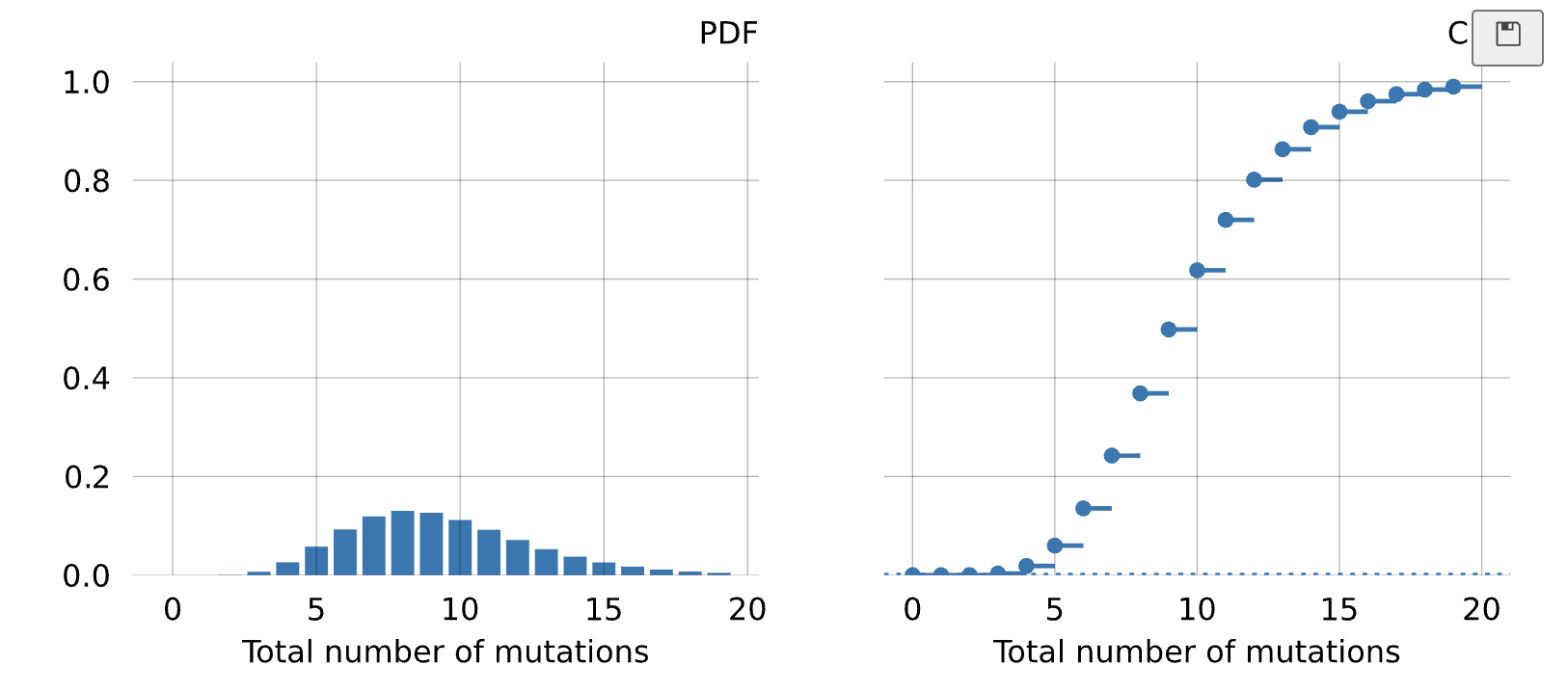
NB: Used to be:

Continuous / Discrete method behavior

The methods moments, expectation, variance, covariance, pdf, cdf, distribution_context, sample, state_probability, and accumulated_occupancy will treat the graph as continuous or discrete in accordance with its is_discrete attribute. In the case moments and probabilities are computed across discrete jumps rather than across continuous time.

It is sometimes useful to interpret a discrete graph as a continuous distribution. However, passing discrete=True to a method called on a continuous will raise a ValueError, since continuous graph has not discrete interpretation.

Methods without the discrete keyword argument, either apply to both kinds of graphs (expected_waiting_time), or automatically redirect to functions handling each kind (normalize, reward_transform).

Multivariate phase-type distributions (marginal)

To produce the discrete marginal expectations we need to discretize the reward-transformed graph:

graph = Graph(coalescent)
rewards = graph.states().T[:-1]
singleton_rewards = rewards[0]

# 1. marginalize
marg_graph = graph.reward_transform(singleton_rewards)

# 2. discretize
disc_marg_graph = marg_graph.discretize(mutation_rate)

disc_marg_graph.plot()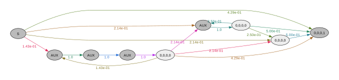

and then pass the unit rewards for the AUX states to compute the expectation:

disc_marg_graph.expectation(disc_marg_graph.rewards)

2.0

Marginalize - then discretize

We must marginalize first and then discretize. If we discretize first, singleton_rewards no longer apply, and even if we find the rewards that marginalize the discretized graph, the rewards attribute of the marginal graph would not be valid.

The expectations for the continuous and discrete distributions are of cause the same, but the variances are different:

graph.variance(), disc_marg_graph.variance(disc_marg_graph.rewards)

(1.1388888888888884, 3.7777777777777786)

To get a graph for the marginal distribution that we can call pdf and cdf on, we just need to reward transform using the same unit rewards we passed to expectation():

marg_mutation_graph = disc_marg_graph.reward_transform(disc_marg_graph.rewards)

marg_mutation_graph.pdf(np.arange(5))

array([0.24   , 0.252  , 0.1932 , 0.12924, 0.07998])

pdf() computes the PMF when called on a graph for a discrete distribution (if the is_discrete attribute is True).

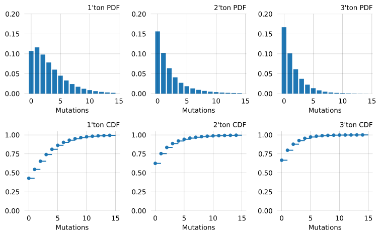
marg_mutation_graph.is_discrete, np.sum(marg_mutation_graph.pdf(np.arange(0, 100))).item()

(True, 0.9999999999999999)

Figure 7 shows the PMF and CDF for each marginal.

fig, axes = plt.subplots(2, len(rewards), figsize=(8, 5))

graph = Graph(coalescent)
rewards = graph.states().T[:-1]
x = np.arange(0, 15)
for i, r in enumerate(rewards):
    rt = graph.reward_transform(r)
    drt = rt.discretize(mutation_rate)
    marg_mutation_graph = drt.reward_transform(drt.rewards)

    pmf = marg_mutation_graph.pdf(x)
    cdf = marg_mutation_graph.cdf(x)

    axes[0, i].set_title(f"{i+1}'ton PDF")
    axes[0, i].bar(x, pmf)
    axes[0, i].set_xlabel('Mutations')
    left, right = x, np.arange(1, x.size+1, 1)
    axes[1, i].hlines(y=cdf, xmin=left, xmax=right, zorder=1)
    axes[1, i].scatter(left, cdf, s=18, zorder=2)
    axes[1, i].set_title(f"{i+1}'ton CDF")
    axes[1, i].set_xlabel('Mutations')
    axes[1, i].set_ylim(0, 1.05)
    
plt.tight_layout()