import phasic
from phasic import (
    Graph, with_ipv, SVGD, GaussPrior, ExpStepSize, Adamelia,
    clear_caches, set_log_level, StateIndexer, Property,
    model_selection,
)
phasic.configure(parallel_elimination=True, reward_compute_cache=True)

from itertools import combinations_with_replacement
from functools import partial
import numpy as np
import jax.numpy as jnp
import matplotlib.pyplot as plt
all_pairs = partial(combinations_with_replacement, r=2)
np.random.seed(42)

from vscodenb import set_vscode_theme
set_vscode_theme()AIC, BIC, LR test
Phasic provides three classical model-selection recipes: Akaike Information Criterion (AIC) and Bayesian Information Criterion (BIC) for ranking models on a parsimony/fit tradeoff and likelihood-ratio test for comparing nested models. They consume the same three quantities available in the fitted SVGD instance:
svgd.log_likelihood()— the maximum log-likelihood \(\log \hat L = \sum_i \log p(x_i \mid \hat\theta)\) at the MAP.svgd.degrees_of_freedom— the number \(k\) of free parameters (theta_dimminus the number fixed viafixed=).svgd.n_observations— the effective sample size \(n\) (number of non-NaN entries for dense data, orlen(values)forSparseObservations).
def two_locus_ghost_island(state, indexer=None):

    coef_len = 6

    pop1_coal_idx = 0
    pop1_rec_idx = 1
    pop1_mig_idx = 2
    pop2_coal_idx = 3
    pop2_rec_idx = 4
    pop2_mig_idx = 5

    transitions = []

    nonzero_idx = np.nonzero(state[:indexer.descendants.state_length])[0]

    if state.sum() <= 1: return transitions

    for i, j in all_pairs(nonzero_idx):

    # for i in range(indexer.state_length):
        if state[i] == 0: continue
        props_i = indexer.descendants.index_to_props(i)

        # for j in range(i, indexer.state_length):
        if state[j] == 0: continue
        props_j = indexer.descendants.index_to_props(j)

        if props_j.in_pop != props_i.in_pop:
            # skip if in different pops
            continue

        same = int(i == j)
        if same and state[i] < 2:
            # skip if same and less than two lineages
            continue
        if not same and (state[i] < 1 or state[j] < 1):
            # skip if different and either kind has no lineages
            continue

        # coalescence
        loc1=props_i.loc1 + props_j.loc1
        loc2=props_i.loc2 + props_j.loc2
        if loc1 <= nr_samples and loc2 <= nr_samples:
            child = state.copy()
            child[i] -= 1
            child[j] -= 1
            k = indexer.descendants.props_to_index(
                loc1=props_i.loc1 + props_j.loc1,
                loc2=props_i.loc2 + props_j.loc2,
                in_pop=props_i.in_pop
                )
            child[k] += 1
            # validate(child, indexer, state)

            coef = np.zeros(coef_len) # +1 to have a slot for transitions between epochs
            if props_i.in_pop == 1:
                coef[pop1_coal_idx] = state[i]*(state[j]-same)/(1+same)
            else:
                coef[pop2_coal_idx] = state[i]*(state[j]-same)/(1+same)
            transitions.append([child, coef])

            # transitions.append([child, [state[i]*(state[j]-same)/(1+same), 0, 0]])

    for i in nonzero_idx:
        props_i = indexer.descendants.index_to_props(i)

        # recombination
        loc1 = props_i.loc1
        loc2 = props_i.loc2
        if state[i] > 0 and 0 < loc1 <= nr_samples and 0 < loc2 <= nr_samples:
            child = state.copy()
            child[i] -= 1
            k = indexer.descendants.props_to_index(
                loc1=0,
                loc2=props_i.loc2,
                in_pop=props_i.in_pop
                )
            child[k] += 1
            k = indexer.descendants.props_to_index(
                loc1=props_i.loc1,
                loc2=0,
                in_pop=props_i.in_pop
                )
            child[k] += 1
            # validate(child, indexer, state)
            coef = np.zeros(coef_len) # +1 to have a slot for transitions between epochs
            if props_i.in_pop == 1:
                coef[pop1_rec_idx] = state[i]
            else:
                coef[pop2_rec_idx] = state[i]
            transitions.append([child, coef])
#            transitions.append([child, [0, state[i], 0]])

        # migration
        if state[i] > 0:
            child = state.copy()
            other_pop = 2 if props_i.in_pop == 1 else 1
            child = state.copy()
            child[i] -= 1
            k = indexer.descendants.props_to_index(
                loc1=props_i.loc1,
                loc2=props_i.loc2,
                in_pop=other_pop
                )
            child[k] += 1
            # validate(child, indexer, state)
            coef = np.zeros(coef_len) # +1 to have a slot for transitions between epochs
            if props_i.in_pop == 2:
                 coef[pop1_mig_idx] = state[i]
            else:
                coef[pop2_mig_idx] = state[i]
            transitions.append([child, coef])
            # transitions.append([child, [0, 0, state[i]]])

    return transitions

nr_samples = 2
true_theta = [
    # pop1_coal, pop1_rec, pop1_mig,
    1, 1, 3,
    # pop2_coal, pop2_rec, pop2_mig
    1, 1, 3,
]
mutation_rate = 0.1
reward_limit = 1

indexer = StateIndexer(
    descendants=[
        Property('loc1', min_value=0, max_value=nr_samples),
        Property('loc2', min_value=0, max_value=nr_samples),
        Property('in_pop', min_value=1, max_value=2),
    ],
)
indexer.state_length
initial = [0] * indexer.state_length
initial[indexer.descendants.props_to_index(loc1=1, loc2=1, in_pop=1)] = nr_samples

graph = Graph(two_locus_ghost_island, ipv=initial, indexer=indexer)
graph.update_weights(true_theta)

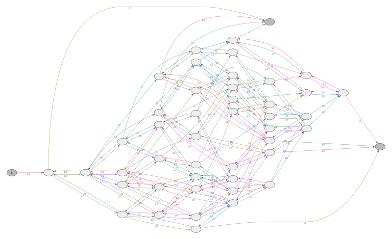
graph.plot(nodesep=0.4, ranksep=2, max_nodes=200,
           label_fmt=False, size=(8,8),
           )
jp_graph = graph.joint_prob_graph(reward_limit=reward_limit,
                                  mutation_rate=mutation_rate)
jp_graph.vertices_length()5380jp_graph.update_weights(true_theta + [mutation_rate])
joint_prob_table = jp_graph.joint_prob_table()
(1 - joint_prob_table['prob'].sum()).item()0.008802869841632588def sample_joint_observations(joint_prob_graph, theta, nr_observations):
joint_prob_graph.update_weights(theta)
joint_prob_table = joint_prob_graph.joint_prob_table()
p = joint_prob_table['prob'] / joint_prob_table['prob'].sum()
p = p.to_numpy()
sample = np.random.choice(joint_prob_table.index.values, nr_observations, p=p)
observations = joint_prob_table.loc[sample, joint_prob_table.columns[:-1]].to_numpy().tolist()
return observations
observations = sample_joint_observations(jp_graph, true_theta + [mutation_rate], nr_observations=1000)
observations[:5][[0, 0, 0, 0, 0, 0, 0, 0],
[0, 1, 0, 0, 0, 0, 0, 1],
[0, 0, 0, 0, 0, 0, 0, 0],
[0, 0, 0, 0, 0, 0, 0, 0],
[0, 0, 0, 0, 0, 0, 0, 0]]jp_graph = graph.joint_prob_graph(reward_limit=reward_limit,
mutation_rate=mutation_rate) %%monitor
svgd = jp_graph.svgd(
observations,
preconditioner='none',
prior=GaussPrior(ci=[0.1, 7]),
n_iterations=50,
n_particles=50,
optimizer=Adamelia(learning_rate=0.2),
fixed=[(3, mutation_rate)],
progress=True,
)
svgd.summary() Parameter Fixed MAP Mean SD HPD 95% lo HPD 95% hi
0 No 5.683 2.381 1.96 0.1737 6.086
1 No 2.942 3.54 1.062 1.673 5.237
2 No 0.9952 1.705 0.804 0.6831 3.392
3 Yes 0.1 NA NA NA NA
4 No 0.187 1.01 0.6587 0.02215 2.087
5 No 3.843 6.924 1.797 3.843 9.391
6 No 0.082 1.778 0.9772 0.005796 2.894
Particles: 50, Iterations: 50# print(f"log L̂ = {svgd.log_likelihood(refine=True):.4f}")
print(f"log L̂ = {svgd.log_likelihood(refine=False):.4f}")
print(f"k (free params) = {svgd.degrees_of_freedom}")
print(f"n (obs) = {svgd.n_observations}")log L̂ = -1556.5178
k (free params) = 6
n (obs) = 1000AIC and BIC for a single fit
refine=True runs a short gradient-ascent refinement of the MAP particle on the log-posterior before evaluating the log-likelihood. The result is closer to the MLE under weak priors and gives a sharper AIC/BIC.
# print(model_selection.aic(svgd, refine=True))
# print(model_selection.bic(svgd, refine=True))
print(model_selection.aic(svgd, refine=False))
print(model_selection.bic(svgd, refine=False))
AICResult(aic=3125.0357, log_likelihood=-1556.5178, k=6, n=1000, refined=False)
BICResult(bic=3154.4822, log_likelihood=-1556.5178, k=6, n=1000, refined=False)Model comparison
Same model but fitting separate coalescence rates for each epoch. If you want to compare models using AIC or BIC, you can fit this model just like the one above. However, to allow an LR test of nested models, you must make the fits on the same model only changing the fixed or tied kwargs. You can extract and reuse the model like this:
svgd_no_mig = SVGD(
    model=svgd.model,
    theta_dim=svgd.theta_dim,
    # Reuse the *processed* observations from the first fit — for a joint-prob
    # model these are the per-observation positions, not the raw 2D array.
    observed_data=svgd.observed_data,
    preconditioner='none',
    prior=GaussPrior(ci=[0.1, 7]),
    n_iterations=50,
    n_particles=50,
    optimizer=Adamelia(learning_rate=0.2),
    fixed=[(1, 0), (3, mutation_rate)],
    progress=True,
)
svgd_no_mig.optimize()
svgd_no_mig.summary()
# print(f"log L̂ = {svgd_all_coal_free.log_likelihood(refine=True):.4f}")
print(f"log L̂ = {svgd_no_mig.log_likelihood(refine=False):.4f}")
print(f"k (free params) = {svgd_no_mig.degrees_of_freedom}")
print(f"n (obs) = {svgd_no_mig.n_observations}")# print(model_selection.aic(svgd_no_mig, refine=True))
# print(model_selection.bic(svgd_no_mig, refine=True))
print(model_selection.aic(svgd_no_mig, refine=False))
print(model_selection.bic(svgd_no_mig, refine=False))Compare the two models:
table = model_selection.compare(
    ("with-migration", svgd),
    ("no-migration", svgd_no_mig),
    criterion='aic',
    # refine=True,
    refine=False,
)
print(table)
Reading the table:
- Rows are sorted ascending by AIC — the best model is on top.
Δis the AIC difference from the best model. Rules of thumb (Burnham & Anderson): Δ < 2 means “essentially equivalent”, 4–7 means “considerably less support”, > 10 means “essentially no support”.weightis the Akaike weight \(\exp(-\Delta_i / 2) / \sum_j \exp(-\Delta_j / 2)\) — the probability, under the AIC/Kullback–Leibler approximation, that model \(i\) is the best of the set.
The one-rate model wins AIC even though the data were generated from the two-rate model. With Δ ≈ 1.6 between the two, the data are not strong enough to justify the extra parameter — AIC is doing exactly the job it should. The three-rate model is meaningfully worse (Δ ≈ 3.6), which is reassuring: the spurious extra parameter is being penalized.
Switch to BIC for a more aggressive complexity penalty:
print(model_selection.compare(
    ("with-migration", svgd),
    ("no-migration", svgd_no_mig),
    criterion='bic',
    # refine=True,
    refine=False,
))
Likelihood-ratio test for nested models
Information criteria rank models that may or may not be nested. When you have a truly nested restriction (the nested model fixes some parameters of the full model at specific values), the likelihood-ratio test gives a frequentist p-value under the null hypothesis that the restriction holds:
\[ 2 \bigl( \log \hat L_\mathrm{full} - \log \hat L_\mathrm{nested} \bigr) \;\sim\; \chi^2_{\,k_\mathrm{full} - k_\mathrm{nested}} \]
Phasic enforces strict nesting: both fits must use the same model callable (the closure returned by one call to Graph.pmf_and_moments_from_graph), the same theta_dim, the same number of observations, and the nested fit’s fixed set must be a strict superset of the full fit’s fixed set. That’s exactly the relationship between svgd (migration free, fixed=[(3, mutation_rate)]) and svgd_no_mig (migration fixed to zero, fixed=[(1, 0), (3, mutation_rate)]):
# Full = svgd (migration free); nested = svgd_no_mig (migration fixed to 0).
# svgd_no_mig's fixed set is a strict superset of svgd's, so they're nested.
lrt = model_selection.likelihood_ratio_test(svgd, svgd_no_mig)
print(lrt)
If the p-value is small (the conventional cutoff is 0.05), the data reject the one-rate restriction — the full two-rate model fits significantly better. A large p-value means the restriction is consistent with the data and the simpler one-rate model can be retained.
In our example p ≈ 0.51 — the test fails to reject the one-rate restriction, in agreement with the AIC/BIC ranking. This is the typical outcome when the two rates are similar relative to the sample size: the likelihood under the two-rate fit is barely better than under the one-rate fit, the statistic 2·(LL_full − LL_nested) is small, and χ²₁ assigns it a large p-value.
Continuous time epoch models
cjp_graph = graph.joint_prob_graph(reward_limit=reward_limit,
                                          mutation_rate=mutation_rate,
discrete=False) # <-- NB! set_log_level('DEBUG')%%monitor
svgd_all_tied = cjp_graph.svgd(
observations,
preconditioner='none',
prior=GaussPrior(ci=[0.1, 7]),
# n_iterations=20,
# n_particles=20,
n_iterations=100,
n_particles=50,
optimizer=Adamelia(learning_rate=0.2),
fixed=[(3, mutation_rate)],
epoch_starts=[0, 0.5],
tied=[
(0, [0, 1]), # tie coal rate in epoch 0 and 1
(1, [0, 1]), # tie rec rate in epoch 0 and 1
(2, [0, 1]), # tie mig rate in epoch 0 and 1.
],
daisy_chain_t_eval='auto',
# daisy_chain_granularity=50,
progress=True,
)
svgd_all_tied.summary() # print(f"log L̂ = {svgd_all_tied.log_likelihood(refine=True):.4f}")
print(f"log L̂ = {svgd_all_tied.log_likelihood(refine=False):.4f}")
print(f"k (free params) = {svgd_all_tied.degrees_of_freedom}")
print(f"n (obs) = {svgd_all_tied.n_observations}")# print(model_selection.aic(svgd_all_tied, refine=True))
# print(model_selection.bic(svgd_all_tied, refine=True))
print(model_selection.aic(svgd_all_tied, refine=False))
print(model_selection.bic(svgd_all_tied, refine=False))Same model but fitting separate coalescence rates for each epoch. If you want to compare models using AIC or BIC, you can fit this model just like the one above. However, to allow an LR test of nested models, you must make the fits on the same model only changing the fixed or tied kwargs. You can extract and reuse the model like this:
%%monitor

svgd_all_coal_free = SVGD(
    model=svgd_all_tied.model,
    # Reuse the processed observations from the tied fit (not the raw array).
    observed_data=svgd_all_tied.observed_data,
    preconditioner=None,
    prior=GaussPrior(ci=[0.1, 7]),
    # n_iterations=20,
    # n_particles=20,
    n_iterations=2,
    n_particles=5,
    optimizer=Adamelia(learning_rate=0.2),
    epoch_starts=[0, 0.5],
    tied=[
        # (0, [0, 1]), # tie coal rate in epoch 0 and 1  <--- Commented out to fit a coal rate per epoch
        (1, [0, 1]), # tie rec  rate in epoch 0 and 1
        (2, [0, 1]), # tie mig  rate in epoch 0 and 1.
    ],
    fixed=[(3, mutation_rate)],
    progress=True,
)
svgd_all_coal_free.optimize()
svgd_all_coal_free.summary()
# print(f"log L̂ = {svgd_all_coal_free.log_likelihood(refine=True):.4f}")
print(f"log L̂ = {svgd_all_coal_free.log_likelihood(refine=False):.4f}")
print(f"k (free params) = {svgd_all_coal_free.degrees_of_freedom}")
print(f"n (obs) = {svgd_all_coal_free.n_observations}")# print(model_selection.aic(svgd_all_coal_free, refine=True))
# print(model_selection.bic(svgd_all_coal_free, refine=True))
print(model_selection.aic(svgd_all_coal_free, refine=False))
print(model_selection.bic(svgd_all_coal_free, refine=False))table = model_selection.compare(
("separate-coal-rate-per-epoch", svgd_all_coal_free),
("all-params-tied-across-epochs", svgd_all_tied),
criterion='aic',
# refine=True,
refine=False,
)
print(table)print(model_selection.compare(
("separate-coal-rate-per-epoch", svgd_all_coal_free),
("all-params-tied-across-epochs", svgd_all_tied),
criterion='bic',
# refine=True,
refine=False,
))lrt = model_selection.likelihood_ratio_test(svgd_all_coal_free, svgd_all_tied)
print(lrt)