from phasic import (
Graph, with_ipv, GaussPrior, HalfCauchyPrior, LogGaussPrior,
Adam, Adamelia, ExpStepSize, ExpRegularization, clear_caches,
clear_jax_cache, clear_model_cache,
StateIndexer, Property, PropertySet, set_log_level
)
set_log_level('WARNING')
import sys
import numpy as np
import jax.numpy as jnp
import pandas as pd
from typing import Optional
import matplotlib.pyplot as plt
from matplotlib.colors import LogNorm
import seaborn as sns
from tqdm.auto import tqdm
from typing import Optional, Callable
from functools import partial
from itertools import combinations, combinations_with_replacement
from vscodenb import set_vscode_theme
sns.set_palette('tab10')
set_vscode_theme()
all_pairs = partial(combinations_with_replacement, r=2)
np.random.seed(17)
_pytest = "pytest" in sys.modules
# set_log_level('DEBUG')Joint probability inference
Discrete feature joint probability
If you have access to marginal features like counts of mutations shared by your samples (singletons, doubletons etc.), You can compute the joint probability of such events exactly.
Coalescent
nr_samples = 4
indexer = StateIndexer(
lineage=[
Property('descendants', min_value=1, max_value=nr_samples),
]
)
@with_ipv([nr_samples]+[0]*(nr_samples-1))
def coalescent_1param(state, indexer=None):
transitions = []
for i, j in all_pairs(indexer.lineage):
p1 = indexer.lineage.index_to_props(i)
p2 = indexer.lineage.index_to_props(j)
same = int(i == j)
if same and state[i] < 2:
continue
if not same and (state[i] < 1 or state[j] < 1):
continue
new = state.copy()
new[i] -= 1
new[j] -= 1
descendants = p1.descendants + p2.descendants
k = indexer.lineage.props_to_index(descendants=descendants)
new[k] += 1
transitions.append([new, [state[i]*(state[j]-same)/(1+same)]])
return transitions
Step one is to construct the model graph.
graph = Graph(coalescent_1param, indexer=indexer)
graph.plot()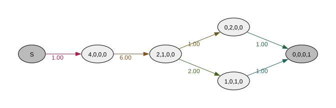
From the model graph we can now create an augmented discrete graph that allow us to compute joint probabilities. This graph is generated for this purpose only and does not otherwise represent the original model. The trick is to track all combinations of events. Each combination is represented by a state with the absorbing one as its only child making each of them the last state in a path through the graph. The probability of passing through one such state thus represents a joint probability. Because we cannot model infinitely many combinations of discrete events, we cap the number of allowed events and route all additional events to an infinite loop not contributing to any joint probability thus defining the distributions deficit.
Controls
reward_limit = 5
mutation_rate = 1e-4
pop_size = 10_000
theta = 1/pop_sizejoint_prob_graph = graph.joint_prob_graph(indexer,
reward_limit=reward_limit,
mutation_rate=mutation_rate)
joint_prob_graph.vertices_length()514Note that the edges now have, not one, but two coefficients. The extra one holds a value scaling the mutation rate.
joint_prob_graph.param_length()2Update edge weights to make the model reflect our true parameter values:
true_theta = [theta, mutation_rate]
joint_prob_graph.update_weights(true_theta)
joint_prob_graph.plot(nodesep=0.3)Graph has too many nodes (514). Please set max_nodes to a higher value.Compute the joint probabilities:
joint_prob_table = joint_prob_graph.joint_prob_table()
joint_prob_table| descendants_1 | descendants_2 | descendants_3 | descendants_4 | prob | |
|---|---|---|---|---|---|
| t_vertex_index | |||||
| 9 | 0 | 0 | 0 | 0 | 9.996334e-01 |
| 19 | 0 | 1 | 0 | 0 | 9.994669e-05 |
| 21 | 1 | 0 | 0 | 0 | 1.999023e-04 |
| 24 | 0 | 0 | 1 | 0 | 6.662890e-05 |
| 36 | 0 | 2 | 0 | 0 | 1.665434e-08 |
| ... | ... | ... | ... | ... | ... |
| 505 | 3 | 5 | 5 | 0 | 6.940044e-53 |
| 506 | 5 | 4 | 5 | 0 | 1.485583e-55 |
| 507 | 5 | 5 | 4 | 0 | 4.186802e-56 |
| 509 | 4 | 5 | 5 | 0 | 2.297372e-56 |
| 510 | 5 | 5 | 5 | 0 | 6.482878e-60 |
216 rows × 5 columns
ax = plt.subplot(111)
ax.axhline(1, c='red', ls=':', lw=1)
ax.plot(joint_prob_table.prob.cumsum()) ;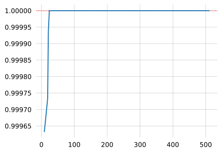
Deficit:
(1 - joint_prob_table['prob'].sum()).item()2.220446049250313e-16Test data
For testing and demonstration purposes, we can sample observations from the model.
def sample_joint_observations(joint_prob_graph, theta, nr_observations):
joint_prob_graph.update_weights(theta)
joint_prob_table = joint_prob_graph.joint_prob_table()
p = joint_prob_table['prob'] / joint_prob_table['prob'].sum()
p = p.to_numpy()
sample = np.random.choice(joint_prob_table.index.values, nr_observations, p=p)
observations = joint_prob_table.loc[sample, joint_prob_table.columns[:-1]].to_numpy().tolist()
return observationstrue_theta = [theta, mutation_rate] # coalescent rate and mutation rate
observations = sample_joint_observations(joint_prob_graph, true_theta, nr_observations=10000)
observations[:5][[0, 0, 0, 0], [0, 0, 0, 0], [0, 0, 0, 0], [0, 0, 0, 0], [0, 0, 0, 0]]For real data, make sure to only to include observations that are possible under the model:
modelled_obs = joint.loc[sample, joint.columns[:-1]].to_numpy().tolist()
allowed_observations = set(tuple(x) for x in modelled_obs)
observations = [o for o in observations if tuple(o) in allowed_observations]
observations = np.array(observations)
observationslearning_rate = ExpStepSize(first_step=0.05, last_step=0.005, tau=30.0)
learning_rate.plot(200) ;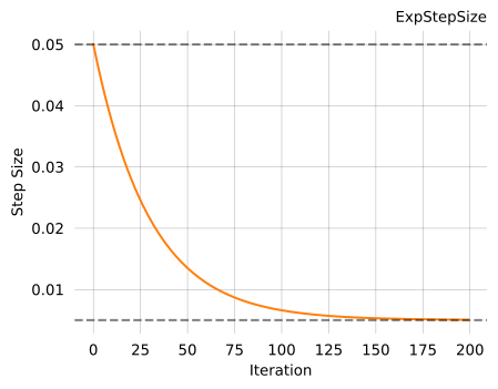
from phasic import LogGaussPrior
LogGaussPrior(ci=[1/100_000, 1/5000]).plot() ;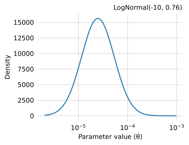
svgd = joint_prob_graph.svgd(
observations,
fixed=[(1, mutation_rate)],
prior=LogGaussPrior(ci=[1/50_000, 1/5000]),
n_iterations=200,
# n_particles=20,
optimizer=Adamelia(learning_rate=0.2),
# learning_rate=learning_rate,
)svgd.summary(ci_method='hpd', ci_level=0.95)Parameter Fixed MAP Mean SD HPD 95% lo HPD 95% hi
0 No 9.062e-05 9.523e-05 9.113e-06 8.418e-05 0.0001149
1 Yes 0.0001 NA NA NA NA
Particles: 40, Iterations: 200svgd.plot_ci(ci_method='hpd')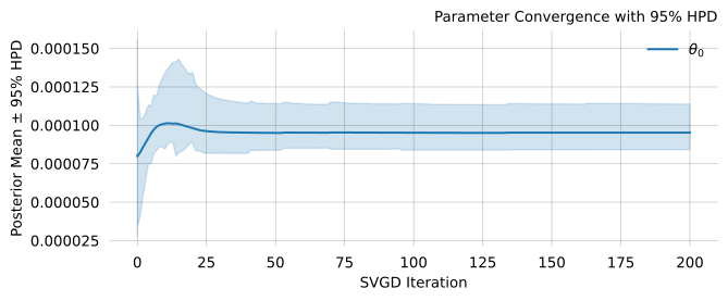
svgd.plot_convergence()
svgd.plot_trace()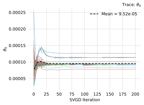
Epoch-wise time-inhomogeneous models
If construct the joint probability graph using discrete=False, you can pass the epoch_starts keyword argument to SVGD to supply a list of epoch start times, SVGD will estimate a set of parameters for each epoch. Note that the the first epoch start must always be zero. E.g., epoch_starts=[0, 0.5] specifies two epochs. One starting at time zero and one starting at time 0.5.
graph = Graph(coalescent_1param, indexer=indexer)
joint_prob_graph = graph.joint_prob_graph(reward_limit=reward_limit,
mutation_rate=mutation_rate,
discrete=False) # <-- NB!
svgd = joint_prob_graph.svgd(
observations,
preconditioner=None,
fixed=[(1, mutation_rate)],
prior=LogGaussPrior(ci=[1/50_000, 1/5000]),
n_iterations=20,
# n_particles=20,
optimizer=Adamelia(learning_rate=0.2),
epoch_starts=[0, 0.5], # <-- NB!
)
svgd.summary(ci_method='hpd', ci_level=0.95)Parameter Fixed MAP Mean SD HPD 95% lo HPD 95% hi
0 No 6.037e-05 6.449e-05 6.716e-06 5.61e-05 8.252e-05
1 Yes 0.0001 NA NA NA NA
2 No 8.938e-05 9.617e-05 7.687e-06 7.31e-05 0.0001027
3 Yes 0.0001 NA NA NA NA
Particles: 80, Iterations: 20svgd.plot_ci(ci_method='hpd')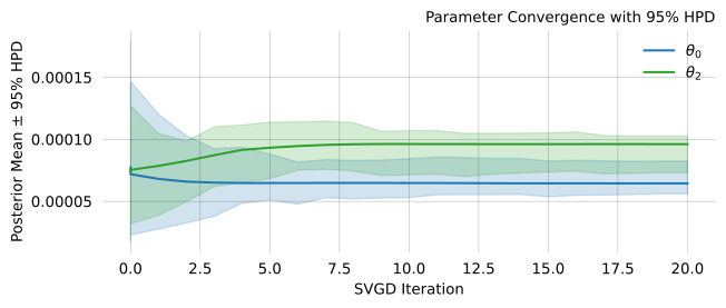
svgd.plot_convergence()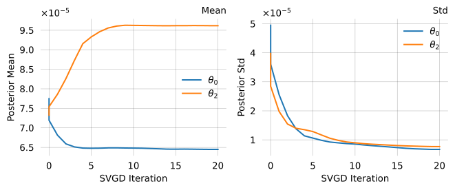
from phasic import Graph, with_ipv, ExpStepSize, LogGaussPrior, StateIndexer, Property
import msprime
import numpy as np
from functools import partial
from itertools import combinations_with_replacement
all_pairs = partial(combinations_with_replacement, r=2)
from vscodenb import set_vscode_theme
set_vscode_theme()
# import phasic
# phasic.set_log_level('DEBUG') # gives phasic-side progress
# # In your call, also enable JAX-side compile logs:
# import os
# os.environ['JAX_LOG_COMPILES'] = '1'
reward_limit = 5
mut_rate = 1.0e-8
rec_rate = 1e-8
nr_samples = 8
seq_length = 10_000_000
# epoch_starts = [0, 0.05371094, 0.15234375]
# epoch_pop_sizes = [10_000, 1_000, 10_000]
epoch_starts = [0, 0.2]
epoch_pop_sizes = [10_000, 10_000]
demography = msprime.Demography()
demography.add_population(name="pop", initial_size=epoch_pop_sizes[0])
for s, t in zip(epoch_starts[1:], epoch_pop_sizes[1:]):
demography.add_population_parameters_change(time=t, initial_size=s, population="pop")
ts = msprime.sim_ancestry(samples={"pop": nr_samples}, ploidy=1,
demography=demography, recombination_rate=rec_rate,
sequence_length=seq_length, random_seed=42)
ts = msprime.sim_mutations(ts, rate=mut_rate, random_seed=42)
observations = []
tree_spans = []
for i, tree in enumerate(ts.trees()):
obs = np.zeros(nr_samples)
obs = list(map(int, obs))
obs[-1] = 0
for site in tree.sites():
for mut in site.mutations:
ton = len(list(tree.get_leaves(mut.node)))
obs[ton-1] += 1
# only data with joint computed probs
if obs[-1] or max(obs) > reward_limit:
continue
observations.append(obs)
start, end = tree.interval
tree_spans.append(end - start)
tree_spans = np.array(tree_spans)
# rounding
# tree_spans = tree_spans // 1000 * 1000
# round in log space
base = 2
tree_spans = base**(np.round(np.log(tree_spans)/np.log(base)))
# print('SETTING ALL TREE SPANS TO SAME VALUE')
# tree_spans = np.array([10000]*len(tree_spans))
print('unique tree spans (rounded):', np.unique(tree_spans).size)
def coalescent(state, indexer=None):
transitions = []
for i, j in all_pairs(indexer.lineage):
p1 = indexer.lineage.index_to_props(i)
p2 = indexer.lineage.index_to_props(j)
same = int(i == j)
if same and state[i] < 2:
continue
if not same and (state[i] < 1 or state[j] < 1):
continue
new = state.copy()
new[i] -= 1
new[j] -= 1
descendants = p1.descendants + p2.descendants
k = indexer.lineage.props_to_index(descendants=descendants)
new[k] += 1
transitions.append([new, [state[i]*(state[j]-same)/(1+same)]])
return transitions
indexer = StateIndexer(
lineage=[
Property('descendants', min_value=1, max_value=nr_samples),
]
)
initial = np.zeros(indexer.state_length, dtype=int)
initial[indexer.p2i(descendants=1)] = nr_samples
initial = initial.tolist() # SHOULD NOT BE NECESSARY AFTER FIXING ISSUE 26
graph = Graph(coalescent, ipv=initial, indexer=indexer)
joint_prob_graph_cont = graph.joint_prob_graph(
indexer, reward_limit=reward_limit,
mutation_rate=mut_rate, discrete=False
)unique tree spans (rounded): 14svgd = joint_prob_graph_cont.svgd(
observations,
preconditioner=None,
fixed=[(1, mut_rate)],
prior=LogGaussPrior(ci=[1/50_000, 1/2000]), # WITHOUT A PRIOR IT HANGS... MAYBE BECAUSE THE NORMAL MOMENTS-BASED SCHEME IS NOT AVAILABLE FOR JOINT GRAPHS
learning_rate=ExpStepSize(first_step=0.05, last_step=0.005, tau=30.0),
epoch_starts=epoch_starts,
exposure=tree_spans,
exposure_param_index=1,
progress=True,
n_iterations=50,
n_particles=20,
# verbose=True,
)/var/folders/s6/srs8qkh52w1_h32d65z95tth0000gn/T/ipykernel_53728/2628073587.py:1: SvgdAssumptionWarning: preconditioner='auto' resolves to the probability-Jacobian preconditioner (built from the model's probability output) for this joint-probability model.
svgd = joint_prob_graph_cont.svgd(--------------------------------------------------------------------------- KeyboardInterrupt Traceback (most recent call last) Cell In[25], line 1 ----> 1 svgd = joint_prob_graph_cont.svgd( 2 observations, 3 preconditioner=None, 4 fixed=[(1, mut_rate)], File ~/phasic/.pixi/envs/default/lib/python3.13/site-packages/phasic/__init__.py:6645, in Graph.svgd(self, observed_data, discrete, prior, n_particles, n_iterations, optimizer, learning_rate, bandwidth, theta_init, theta_dim, return_history, seed, verbose, progress, jit, parallel, n_devices, precompile, compilation_config, regularization, nr_moments, positive_params, param_transform, joint_index, rewards, fixed, tied, callback, weight_formula, preconditioner, epoch_starts, daisy_chain_t_eval, daisy_chain_granularity, daisy_chain_probe_theta, daisy_chain_t_eval_tol, final_read, exposure, exposure_param_index, validate_rewards, quiet_assumptions, exact_moment_grad, exact_final_grad, exact_grad) 6641 # path). 6642 if _callback_overridden: 6643 self._weight_callback = _prev_weight_callback 6644 self._weight_mode = _prev_weight_mode -> 6645 if _formula_overridden: 6646 self._restore_weight_formula_state(*_prev_formula_state) File ~/phasic/.pixi/envs/default/lib/python3.13/site-packages/phasic/__init__.py:4384, in Graph._daisy_chain_svgd_model(self, observed_indices, epoch_starts, t_eval, user_prior, user_fixed, user_tied, sd, verbose, granularity, exposure_arr, exposure_param_index, final_read, bake_fd_skip, exact_final_grad) 4380 " graph.joint_prob_graph(indexer, ..., discrete=False)" 4381 ) 4382 4383 # Build the JSP graph and the initial IPV (in JSP-graph IPV-coords). -> 4384 jsp = self.joint_stop_prob_graph() 4385 n_ipv = len(jsp._ipv_target_indices) 4386 # Read self's IPV (length self.vertices_length()) and project to 4387 # the JSP graph's IPV layout. self's IPV has nonzero entries File ~/phasic/.pixi/envs/default/lib/python3.13/site-packages/phasic/__init__.py:10767, in Graph.joint_stop_prob_graph(self) 10763 t_aux_vertex = nv.add_aux_vertex_constant(1.0) 10764 t_aux_map[nv.index()] = t_aux_vertex.index() 10765 continue 10766 > 10767 for e in v.parameterized_edges(): 10768 to_index = e.to().index() 10769 if to_index in trash_old_indices: 10770 to_index = abs_old_index KeyboardInterrupt:
svgd.summary(ci_method='hpd', ci_level=0.95)svgd.summary(ci_method='hpd', ci_level=0.95)Parameter Fixed MAP Mean SD HPD 95% lo HPD 95% hi
0 No 5.134e-05 0.0001043 6.337e-05 8.842e-06 0.0001913
1 Yes 1e-08 NA NA NA NA
2 No 1e-09 8.148e-09 1.883e-08 1e-09 4.18e-08
3 Yes 1e-08 NA NA NA NA
Particles: 20, Iterations: 50svgd.plot_ci(ci_method='hpd')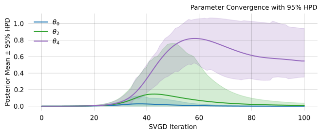
svgd.plot_convergence()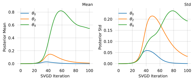
svgd.plot_trace()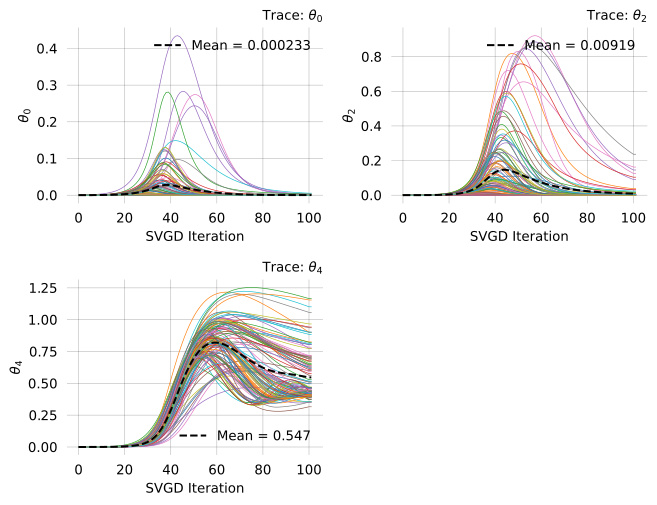
joint_prob_graph_cont = graph.joint_prob_graph(indexer, reward_limit=reward_limit, mutation_rate=mutation_rate,
discrete=False)
svgd = joint_prob_graph_cont.svgd(
observations,
preconditioner='none',
joint_index=True, # map count vectors -> joint-prob table indices
# exposure=tree_spans, # per-observation alpha (e.g. segment length)
# exposure_param_index=1, # which theta slot the exposure scales (the rate)
fixed=[(1, mutation_rate)],
n_iterations=100,
prior=LogGaussPrior(ci=[1/50_000, 1/5000]), # WITHOUT A PRIOR IT HANGS... MAYBE BECAUSE THE NORMAL MOMENTS-BASED SCHEME IS NOT AVAILABLE FOR JOINT GRAPHS
# prior=GaussPrior(ci=[0.5, 5]), # WITHOUT A PRIOR IT HANGS... MAYBE BECAUSE THE NORMAL MOMENTS-BASED SCHEME IS NOT AVAILABLE FOR JOINT GRAPHS
optimizer=Adamelia(learning_rate=0.2),
# learning_rate=learning_rate,
# daisy_chain_t_eval=30,
daisy_chain_t_eval='auto',
# daisy_chain_t_eval_tol=1e-6, # default; tighter = more conservative
# daisy_chain_probe_theta=[5.0, 1.0], # optional; defaults to ones
epoch_starts=[0, 0.05371094, 0.15234375]
)--------------------------------------------------------------------------- KeyboardInterrupt Traceback (most recent call last) Cell In[26], line 3 1 joint_prob_graph_cont = graph.joint_prob_graph(indexer, reward_limit=reward_limit, mutation_rate=mutation_rate, 2 discrete=False) ----> 3 svgd = joint_prob_graph_cont.svgd( 4 observations, 5 preconditioner='none', 6 joint_index=True, # map count vectors -> joint-prob table indices File ~/phasic/.pixi/envs/default/lib/python3.13/site-packages/phasic/__init__.py:6645, in Graph.svgd(self, observed_data, discrete, prior, n_particles, n_iterations, optimizer, learning_rate, bandwidth, theta_init, theta_dim, return_history, seed, verbose, progress, jit, parallel, n_devices, precompile, compilation_config, regularization, nr_moments, positive_params, param_transform, joint_index, rewards, fixed, tied, callback, weight_formula, preconditioner, epoch_starts, daisy_chain_t_eval, daisy_chain_granularity, daisy_chain_probe_theta, daisy_chain_t_eval_tol, final_read, exposure, exposure_param_index, validate_rewards, quiet_assumptions, exact_moment_grad, exact_final_grad, exact_grad) 6641 # path). 6642 if _callback_overridden: 6643 self._weight_callback = _prev_weight_callback 6644 self._weight_mode = _prev_weight_mode -> 6645 if _formula_overridden: 6646 self._restore_weight_formula_state(*_prev_formula_state) File ~/phasic/.pixi/envs/default/lib/python3.13/site-packages/phasic/__init__.py:11493, in Graph._resolve_daisy_chain_t_eval(self, daisy_chain_t_eval, epoch_starts, probe_theta, tol, granularity, verbose) 11489 ) 11490 return t_val 11491 11492 # 'auto' branch: build JSP graph, probe. > 11493 jsp = self.joint_stop_prob_graph() 11494 n_epochs = int(es.size) 11495 param_length = self.param_length() 11496 if probe_theta is None: File ~/phasic/.pixi/envs/default/lib/python3.13/site-packages/phasic/__init__.py:10767, in Graph.joint_stop_prob_graph(self) 10763 t_aux_vertex = nv.add_aux_vertex_constant(1.0) 10764 t_aux_map[nv.index()] = t_aux_vertex.index() 10765 continue 10766 > 10767 for e in v.parameterized_edges(): 10768 to_index = e.to().index() 10769 if to_index in trash_old_indices: 10770 to_index = abs_old_index KeyboardInterrupt:
svgd.summary(ci_method='hpd', ci_level=0.95)Parameter Fixed MAP Mean SD HPD 95% lo HPD 95% hi
0 No 6.294e-05 0.0002331 0.0006738 3.286e-05 0.0008951
1 Yes 0.0001 NA NA NA NA
2 No 6.029e-05 0.009191 0.03332 4.128e-05 0.03743
3 Yes 0.0001 NA NA NA NA
4 No 0.4148 0.5467 0.1925 0.351 0.9422
5 Yes 0.0001 NA NA NA NA
Particles: 120, Iterations: 100svgd.plot_ci(ci_method='hpd')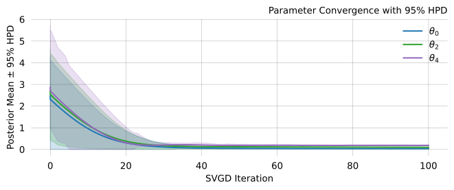
svgd.plot_convergence()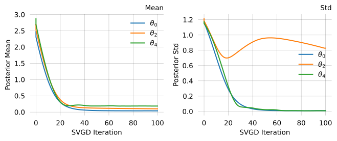
svgd.plot_trace()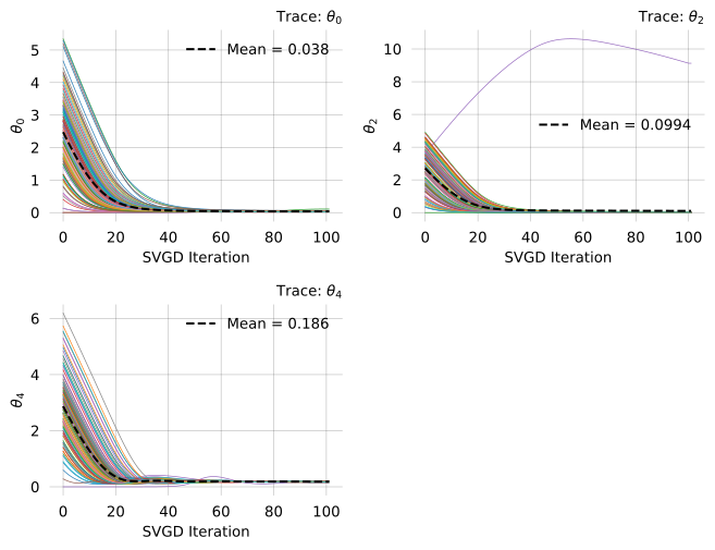
joint_prob_graph_cont = graph.joint_prob_graph(indexer, reward_limit=reward_limit, mutation_rate=mutation_rate,
discrete=False)
svgd = joint_prob_graph_cont.svgd(
observations,
fixed=[(1, mutation_rate)],
n_iterations=100,
prior=GaussPrior(ci=[0.5, 5]), # WITHOUT A PRIOR IT HANGS... MAYBE BECAUSE THE NORMAL MOMENTS-BASED SCHEME IS NOT AVAILABLE FOR JOINT GRAPHS
optimizer=Adamelia(learning_rate=0.2), # WITHOUT A PRIOR IT HANGS... MAYBE BECAUSE THE NORMAL MOMENTS-BASED SCHEME IS NOT AVAILABLE FOR JOINT GRAPHS
# learning_rate=learning_rate,
# daisy_chain_t_eval=30,
daisy_chain_t_eval='auto',
daisy_chain_t_eval_tol=1e-6, # default; tighter = more conservative
# daisy_chain_probe_theta=[5.0, 1.0], # optional; defaults to ones
epoch_starts=[0, 0.05371094, 0.15234375]
)svgd.summary(ci_method='hpd', ci_level=0.95)Parameter Fixed MAP Mean SD HPD 95% lo HPD 95% hi
0 No 0.0376 0.03796 0.01044 0.01966 0.05373
1 Yes 0.0001 NA NA NA NA
2 No 0.02202 0.09938 0.8281 0.0114 0.03982
3 Yes 0.0001 NA NA NA NA
4 No 0.1874 0.1862 0.008462 0.1734 0.2096
5 Yes 0.0001 NA NA NA NA
Particles: 120, Iterations: 100svgd.plot_ci(ci_method='hpd')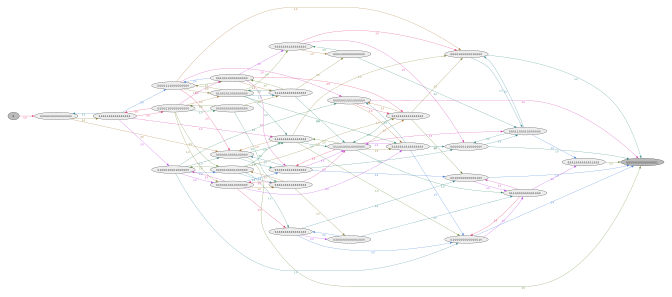
svgd.plot_convergence()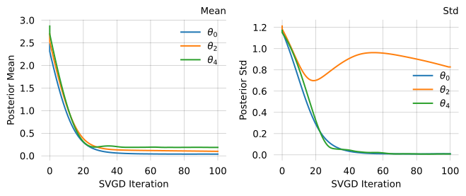
svgd.plot_trace()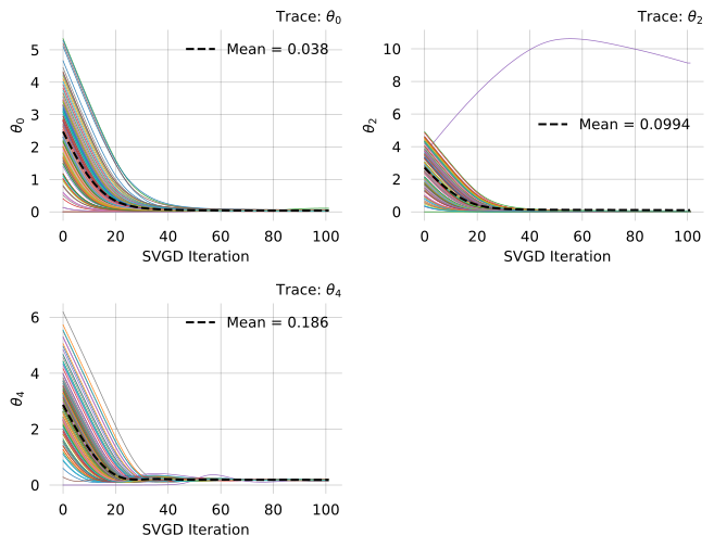
ARG
# create state space for two-locus model
nr_samples = 3
indexer = StateIndexer(
descendants=[
Property('loc1', min_value=0, max_value=nr_samples),
Property('loc2', min_value=0, max_value=nr_samples)
]
)
# initial state with all lineages having one descendant at both loci
initial = [0] * indexer.state_length
initial[indexer.descendants.props_to_index(loc1=1, loc2=1)] = nr_samples
@with_ipv(initial)
def two_locus_arg_2param(state, indexer=None):
transitions = []
if state.sum() <= 1: return transitions
for i in range(indexer.state_length):
if state[i] == 0: continue
props_i = indexer.descendants.index_to_props(i)
for j in range(i, indexer.state_length):
if state[j] == 0: continue
props_j = indexer.descendants.index_to_props(j)
same = int(i == j)
if same and state[i] < 2:
continue
if not same and (state[i] < 1 or state[j] < 1):
continue
child = state.copy()
child[i] -= 1
child[j] -= 1
des_loc1 = props_i.loc1 + props_j.loc1
des_loc2 = props_i.loc2 + props_j.loc2
if des_loc1 <= nr_samples and des_loc2 <= nr_samples:
child[indexer.descendants.props_to_index(loc1=des_loc1, loc2=des_loc2)] += 1
transitions.append([child, [state[i]*(state[j]-same)/(1+same), 0]])
if state[i] > 0 and props_i.loc1 > 0 and props_i.loc2 > 0:
child = state.copy()
child[i] -= 1
child[indexer.descendants.props_to_index(loc1=0, loc2=props_i.loc2)] += 1
child[indexer.descendants.props_to_index(loc1=props_i.loc1, loc2=0)] += 1
transitions.append([child, [0, state[i]]])
# transitions.append([child, [0, 1]])
return transitionsgraph = Graph(two_locus_arg_2param, indexer=indexer,
# graph_cache=True,
# cache_trace=True
)
graph.vertices_length()32graph.plot(nodesep=0.5, wrap=False)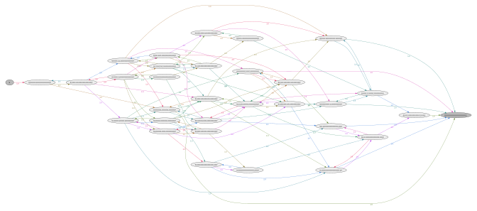
mutation_rate = 1
joint_prob_graph = graph.joint_prob_graph(indexer,
reward_only=['loc1', 'loc2'],
reward_limit=1,
tot_reward_limit=2,
mutation_rate=mutation_rate
)true_theta = [10, 1, mutation_rate] # coalescent, recombination, and mutation rate
observations = sample_joint_observations(joint_prob_graph, true_theta, nr_observations=1000)
observations[:5][[0, 0, 1, 0, 0, 0, 0, 0],
[0, 0, 0, 0, 0, 0, 0, 0],
[0, 1, 0, 0, 0, 1, 0, 0],
[0, 1, 0, 0, 0, 0, 0, 0],
[0, 0, 0, 0, 0, 0, 0, 0]]joint_prob_table = joint_prob_graph.joint_prob_table()
joint_prob_table.head()| loc1_0 | loc1_1 | loc1_2 | loc1_3 | loc2_0 | loc2_1 | loc2_2 | loc2_3 | prob | |
|---|---|---|---|---|---|---|---|---|---|
| t_vertex_index | |||||||||
| 6 | 0 | 0 | 0 | 0 | 0 | 0 | 0 | 0 | 0.576233 |
| 38 | 0 | 1 | 0 | 0 | 0 | 0 | 0 | 0 | 0.088287 |
| 42 | 0 | 0 | 1 | 0 | 0 | 0 | 0 | 0 | 0.040607 |
| 45 | 0 | 0 | 0 | 0 | 0 | 1 | 0 | 0 | 0.088287 |
| 47 | 0 | 0 | 0 | 0 | 0 | 0 | 1 | 0 | 0.040607 |
ExpStepSize(first_step=0.1, last_step=0.01, tau=50.0).plot(100) ;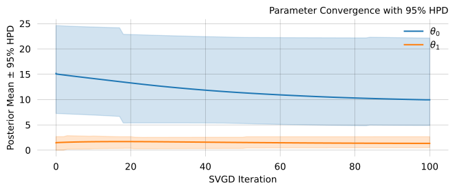
%%monitor
svgd = joint_prob_graph.svgd(
observed_data=observations,
fixed=[(2, mutation_rate)],
n_iterations=100,
n_particles=200,
prior=[
GaussPrior(ci=[5, 25]),
GaussPrior(ci=[0, 3]),
None
],
learning_rate=ExpStepSize(first_step=0.1, last_step=0.01, tau=50.0),
)
svgd.summary()Parameter Fixed MAP Mean SD HPD 95% lo HPD 95% hi
0 No 5.625 9.954 5.399 4.881 22.16
1 No 0.9367 1.345 0.6121 0.4909 2.664
2 Yes 1 NA NA NA NA
Particles: 200, Iterations: 100svgd.plot_ci(ci_method='hpd')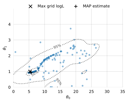
svgd.plot_convergence() ;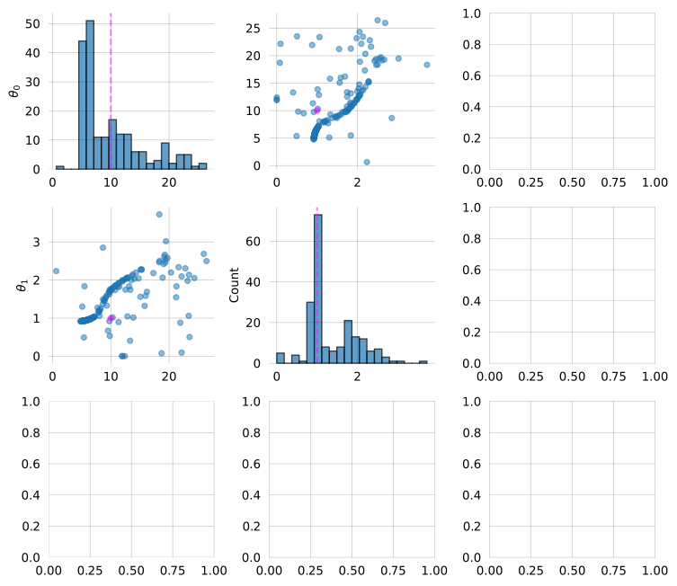
svgd.plot_trace()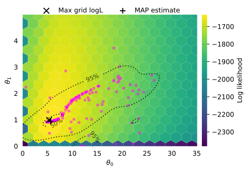
svgd.map_estimate_from_particles()([5.62503240448728, 0.9366762814999638, 1.0], -1631.989130387966)svgd.plot_hdr()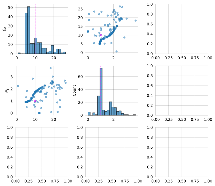
svgd.plot_hdr(hexgrid=False) ;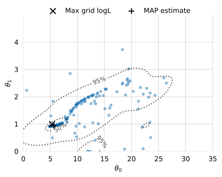
svgd.plot_pairwise(true_theta=true_theta) ;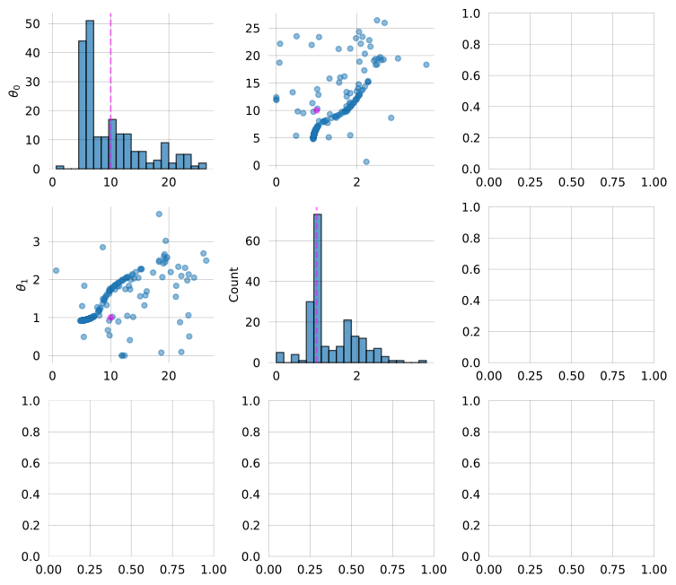
svgd.animate_pairwise(true_theta=true_theta)Example data
Simulation of two-island model:
NB: Simulation requires the msprime and tskit packages, both available as conda packages.
import msprime
import pandas as pd
import numpy as np
import matplotlib.pyplot as plt
%config InlineBackend.figure_format = 'retina'
def derived_counts(ts, rec_rate):
records = []
for var in ts.variants():
p, g = var.site.position, var.genotypes
records.append((int(p), p*rec_rate, g.sum()))
df = pd.DataFrame().from_records(
records, columns=["pos", "gen_pos", "count"]
)
return df
mut_rate = 5e-10
rec_rate = 1e-8
nr_samples = 5
seq_length = 100_000_000
pop1_size, pop2_size, anc_pop_size = 20_000, 10_000, 15_000
migr_pop1_to_pop2 = 1e-4
migr_pop2_to_pop1 = 5e-4
demography = msprime.Demography()
demography.add_population(name="pop1", initial_size=pop1_size)
demography.add_population(name="pop2", initial_size=pop2_size)
demography.set_migration_rate(source="pop1", dest="pop2", rate=migr_pop1_to_pop2)
demography.set_migration_rate(source="pop2", dest="pop1", rate=migr_pop2_to_pop1)
ts = msprime.sim_ancestry(samples={"pop1": nr_samples, "pop2": 0}, ploidy=1,
demography=demography, recombination_rate=rec_rate,
sequence_length=seq_length, random_seed=12)
ts = msprime.sim_mutations(ts, rate=mut_rate, random_seed=5678)
df = derived_counts(ts, rec_rate)
df.to_csv("island_model_derived_counts.csv", index=False)# # isolation with migration (IM) model:
# demography = msprime.Demography()
# demography.add_population(name="pop1", initial_size=pop1_size)
# demography.add_population(name="pop2", initial_size=pop2_size)
# demography.set_migration_rate(source="pop1", dest="pop2", rate=migr_pop1_to_pop2)
# demography.set_migration_rate(source="pop2", dest="pop1", rate=migr_pop2_to_pop1)
# demography.add_population(name="ancestral", initial_size=anc_pop_size)
# demography.add_population_split(time=1000, derived=["pop1", "pop2"], ancestral="ancestral")
# ts = msprime.sim_ancestry(samples={"pop1": nr_samples, "pop2": 0}, ploidy=1,
# demography=demography, recombination_rate=rec_rate,
# sequence_length=seq_length, random_seed=12)
# ts = msprime.sim_mutations(ts, rate=mut_rate, random_seed=5678)
# df = derived_counts(ts, rec_rate)
# df.to_csv("IM_model_derived_counts.csv", index=False)Get pairs of variants in the specified distance range.
def pairs_in_range(nums, diff_lo, diff_hi):
n = len(nums)
lo, hi = 1, 1
pairs = []
for i in range(n):
if lo <= i:
lo = i + 1
while lo < n and nums[lo] - nums[i] < diff_lo:
lo += 1
if hi <= i:
hi = i + 1
while hi < n and nums[hi] - nums[i] <= diff_hi:
hi += 1
for j in range(lo, hi):
pairs.append((i, j))
return pairs
df = pd.read_csv("island_model_derived_counts.csv")
col = "pos" # can also use "gen_pos"
distance, tolerance = 5000, 500
min_dist, max_dist = distance - tolerance, distance + tolerance
records = []
for i, j in pairs_in_range(df[col].values, min_dist, max_dist):
records.append((df.at[i, col], df.at[j, col], df.at[i, "count"], df.at[j, "count"]))
pairs = pd.DataFrame.from_records(records, columns=["pos1", "pos2", "count1", "count2"])
pairs.head()| pos1 | pos2 | count1 | count2 | |
|---|---|---|---|---|
| 0 | 160020 | 164783 | 1 | 3 |
| 1 | 307248 | 311878 | 4 | 1 |
| 2 | 516495 | 521242 | 2 | 1 |
| 3 | 948820 | 953791 | 1 | 3 |
| 4 | 1784175 | 1788903 | 1 | 1 |
We allow multiple SNPs from the same tree, but each SNP can only be part of a single pair. Remove pairs that share a position with another pair:
mask = (pairs.pos1 == pairs.pos1.shift()) | (pairs.pos2 == pairs.pos2.shift())
filtered_pairs = pairs.loc[~mask, :]
filtered_pairs.head()| pos1 | pos2 | count1 | count2 | |
|---|---|---|---|---|
| 0 | 160020 | 164783 | 1 | 3 |
| 1 | 307248 | 311878 | 4 | 1 |
| 2 | 516495 | 521242 | 2 | 1 |
| 3 | 948820 | 953791 | 1 | 3 |
| 4 | 1784175 | 1788903 | 1 | 1 |
Plot position differences for pairs of variants:
plt.hist(filtered_pairs.pos2 - filtered_pairs.pos1, bins=10) ;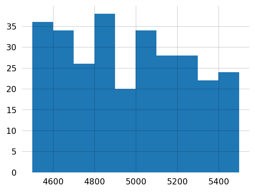
n = len(filtered_pairs)
observations = np.zeros((n, nr_samples), dtype=int)
observations
for i, pair in enumerate(filtered_pairs[["count1", "count2"]].values):
observations[i, pair] = 1msg = f"""
Two-locus observations across {nr_samples} samples of {seq_length/1e6:.0f} Mb:
Mutation rate:
{mut_rate} events/site/generation
Recombination rate:
{rec_rate} crossovers/base/generation
Haploid population sizes:
pop1: {pop1_size}
pop2: {pop2_size}
Migration rate:
pop1 -> pop2: {migr_pop1_to_pop2}
pop2 -> pop1: {migr_pop2_to_pop1}
"""
print(msg)
Two-locus observations across 5 samples of 100 Mb:
Mutation rate:
5e-10 events/site/generation
Recombination rate:
1e-08 crossovers/base/generation
Haploid population sizes:
pop1: 20000
pop2: 10000
Migration rate:
pop1 -> pop2: 0.0001
pop2 -> pop1: 0.0005
Can you make a model and find the true parameters?