Laplace transform

Phase-type distributions

For a phase-type distribution with initial probability vector \(\boldsymbol{\alpha}\) (over the transient states) and sub-intensity matrix \(S\) (the transient block of the generator), the Laplace transform of the absorption time \(\tau\) is

\[\mathbb{E}[e^{-s\tau}] = \boldsymbol{\alpha}(s\boldsymbol{I} - \boldsymbol{S})^{-1}\mathbf{t},\]

where \(\mathbf{t} = -S\mathbf{1}\) is the exit rate vector into the absorbing state. The transform \(\mathbb{E}[e^{-s\tau}]\) is just the expectation of \(e^{-s\tau}\). Formally it is the moment generating function evaluated at \(-s\), so it packages all the moments of the absorption time. Differentiating at \(s=0\) recovers them:

\[ \mathbb{E}[\tau^n] = (-1)^n \frac{d^n}{ds^n}\mathbb{E}[e^{-s\tau}]\big|_{s=0} = n!\,\boldsymbol{\alpha}(-\boldsymbol{S})^{-n}\mathbf{1}. \].

Especially useful is that \(\mathbb{E}[e^{-s\tau}]\) equals the probability that the phase-type process gets absorbed before some independent “killing” event with rate \(s\) occurs (\(\text{Exp}(s)\)). This makes \((s\boldsymbol{I}-\boldsymbol{T})^{-1}_{ij}\) the expected occupation of phase \(j\) before the killing event if starting in \(i\). Multiplying by the exit rates \(\mathbf{t}\) and averaging over the start distribution \(\boldsymbol{\alpha}\) gives the absorption-before-killing probability. As \(s\to 0\) the killing clock never rings, \(\boldsymbol{\alpha}(s\boldsymbol{I} - \boldsymbol{S})^{-1}\) becomes Green matrix \((-\boldsymbol{S})^{-1}\), and the transform goes to 1 meaning that absorption is certain.

from phasic import Graph, with_ipv
import numpy as np
import sys
import matplotlib.pyplot as plt
from matplotlib.colors import LogNorm
import seaborn as sns
from vscodenb import set_vscode_theme
sns.set_palette('tab10')
set_vscode_theme()
np.random.seed(42)

nr_samples = 4

@with_ipv([nr_samples]+[0]*(nr_samples-1))
def coalescent(state):
    transitions = []
    for i in range(state.size):
        for j in range(i, state.size):            
            same = int(i == j)
            if same and state[i] < 2:
                continue
            if not same and (state[i] < 1 or state[j] < 1):
                continue 
            new = state.copy()
            new[i] -= 1
            new[j] -= 1
            new[i+j+1] += 1
            transitions.append((new, state[i]*(state[j]-same)/(1+same)))
    return transitions

Matrix-based computation

Specification in matrix terms:

S = np.array([[-6, 6, 0, 0], 
              [0, -3, 1, 2], 
              [0, 0, -1, 0], 
              [0, 0, 0, -1]], dtype=float)
alpha = np.array([1, 0, 0, 0], dtype=float)  # starting state
n = len(alpha)

Matrix computation of Laplace transform:

theta = 0.5

s0 = -S @ np.ones(n)
laplace_result = np.linalg.solve(theta * np.eye(n) - S, s0)
print(laplace_result)

[0.52747253 0.57142857 0.66666667 0.66666667]

Laplace transform by modifying S:

S_new = S - theta * np.eye(n)
print("Modified S matrix:")
print(S_new)

Modified S matrix:
[[-6.5  6.   0.   0. ]
 [ 0.  -3.5  1.   2. ]
 [ 0.   0.  -1.5  0. ]
 [ 0.   0.   0.  -1.5]]

Laplace transformation as graph operations

In the phasic library, Laplace transform can be implemented by: 1. Adding edges from each transient state to the absorbing state with weight θ 2. Creating a reward vector that is 1 for states with edges to absorption 3. Computing expectations using reward transformation

This is equivalent to the matrix formulation: \(E[e^{-\theta \tau}] = \mathbf{\alpha} (\theta\, \mathbf{I} − \mathbf{S})^{−1}\mathbf{s}\)

graph = Graph(coalescent)
graph.plot()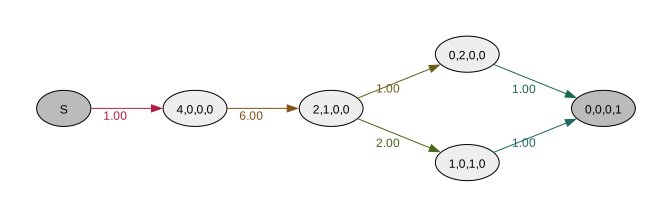

lap_graph = graph.laplace_transform(theta)
lap_graph.plot()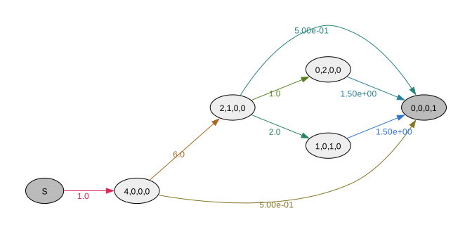

Figure 1

theta = 0.5
rewards = graph.absorbing_state_rewards()
lap_graph.expected_waiting_time(rewards)

[0.5274725274725275,
 0.5274725274725275,
 0.5714285714285714,
 0.6666666666666666,
 0.6666666666666666,
 0.0]

Expectation and Variance

lap_graph.expectation(rewards), lap_graph.variance(rewards)

(0.5274725274725275, 0.4250694360584471)

Higher moments

lap_graph.moments(5)

[0.945054945054945,
 1.4462021494988528,
 3.0644279039400404,
 8.376088953712031,
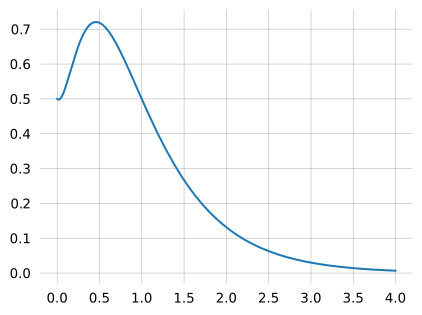
 28.218036661593192]

PDF

time = np.arange(0, 4, 0.001)
pdf = lap_graph.pdf(time)
plt.plot(time, pdf)
plt.show()

Figure 2